Green computing: three examples of how non-trivial mathematical analysis can help

Computing and environment: three directions

Environmental issues are critical for the survival of humankind. These issues are also very complex, with complex dependencies that require computers to solve. This is probably the most important relation between computing and environment: that we need to use computers to solve complicated environment-related problems.

However, there are other relations between environment and computing. One of the most important relations is that computing itself contributes to environmental problems – e.g., by consuming a large amount of energy, energy that mostly comes from the non-renewable energy sources like fossils. To make computing less damaging to the environment, to move towards environment-friendly computing is the second important direction.

Finally, there is a third direction, motivated, in particular, by the success of quantum computing; see, e.g.,^[1]. This success comes largely from the fact that many quantum effects are complex and difficult to predict. This means that by launching some quantum processes and observing the results, we can really fast get the values whose computing on a regular computer would take a long time. In other words, for the corresponding functions, using actual quantum processes leads to faster computation than using a regular computer. It turns out that many of such functions are practically useful – and this, in a nutshell, is what quantum computing is largely about. But environmental processes are also very complex, very difficult to predict – often even more difficult to predict that typical quantum processes. So a natural idea is to use environmental processes for computations. This is the third direction – which may sound promising, but which, at this moment of time, is the least explored.

What we do in this paper

In this paper, we provide three examples that show how non-trivial mathematical analysis can help in all three of these directions: environment-related computing, environment-friendly computing, and environment as computing.

Recycling as an important part of environmental research

There are many important problems in environment-related computing – and we ourselves, together with our students, have participated in solving some of these problems; see, e.g.,^[2-11].

In this section, we will concentrate only on one of these problems – namely, on one of the most fundamental ones. This problem is related to the fact that one of the main reasons why our civilization spends a lot of energy – and thus, contributes to the worsening of the environmental situation – is that we constantly produce new things: clothes, cars, computers, etc. Most of the manufacturing processes consists of several stages on each of which we spend some energy. For example, to produce a computer, we first need energy to extract the ores from the mines, then we need energy to extract the corresponding metals from the ores, we need energy to produce silicon and plastic, then we need energy to combine them into parts, etc.

Each gadget has a limited period of use: cars break down, clothes deteriorate, computers become too slow and obsolete in comparison with the new designs, etc. To save energy – and thus, to save the environment – it is desirable to recycle these gadgets – i.e., to use them to minimize the number of stages need to produce new gadgets. For example, if we melt used aluminum cans into new ones, we do not need energy to extract aluminum from the aluminum ore (and this requires, by the way, a lot of energy).

Recycling is one of the most important issues in environment-related practice.

When is recycling most efficient

The largest amount of savings in recycling is when the material is largely intact, and the only difference between what we have and what we want is the shape of this material. Sometimes, this is part of the manufacturing: for example, when we tailor clothes, we start with material, cut it into appropriate pieces, and sew them together. Sometimes, this is part of recycling: if we have some old clothes in which most material is intact, a tailor can cut it and make new clothes. If we have pieces of clothes which are too small to be useful by themselves, we can sew them together to make a quilt. If we have a metal sheet, and we need to make a tube, we can cut this sheet into pieces and weld them together to form a tube. This is the type of recycling – we will call it geometric recycling – that we will analyze in this section.

Geometric recycling as a mathematical problem

Let us describe this situation in precise geometric terms. We are given an object of certain shape. In mathematical terms, a shape is simply a set of 3-D points, i.e., a subset of the 3-D space . We want to use this object to design an object of a different shape Q. Ideally, we should simply cut the object A into several disjoint pieces

then move these pieces around, so that they form sets Q1,…,Q_p, and combine these sets Q_i into the desired shape Q:

Of course, a generic set is not always a realistic description of a part: for example, we can have weird sets like the set of all rational numbers. To make sure that we consider only practically implementable sets, we need to restrict ourselves, e.g., to polytopes – they approximate any smooth or even non-smooth objects with any needed accuracy, and thus, from the practical viewpoint, represent all possible shapes. So, in the above problem, we assume that the given sets P and Q are polytopes, and that we are looking for polytopes P_i and Q_i.

To perform the above procedure, we need, given two polytopes P and Q, to find the polytopes P_i and Q_i that satisfy the conditions (1) and (2) and for which each polytope Q_i can be obtained from the corresponding polytope P_i by using some shifts and rotations; we will denote this by P_i ~ Q_i. Polytopes P and Q for which such divisions are possible – i.e., which can be composed of “equal” parts P_i ~ Q_i - are called equidecomposable. For each pair (P, Q), the first natural question is: is such a decomposition possible at all?

Of course, rotations and shifts do not change the volume V, so we have V(P_i) = V(Q_i) for all i and thus, V(P) = V(Q). Thus, only sets of equal volume can be equidecomposable. So, this question makes sense only for polytopes of equal volume.

If such a decomposition of P and Q is possible, the next natural question is: what is the smallest number of parts p needed for this process – since the fewer cuts and “glue-ings” we need, the less energy we will spend on this process.

What is known: an early history of this mathematical question

For polygons, the answer to a similar question has been known for some time: every two polygons of equal area are equidecomposable. Since every polygon can be represented as a union of disjoint triangles, this result can be proven if we prove that every triangle is equidecomposable with a right rectangle (2-D box) one of whose sides is equal to 1. This shows that each polygon is equidecomposable with a right rectangle whose one side is 1 and another side is equal to the polygon’s area – and thus, every two polygons with equal area are indeed equidecomposable.

In the 3-D cases, it is reasonable to try the same idea. We can similarly represent each polytope as a union of tetrahedra (= triangular pyramids), but it is not clear whether each tetrahedron is equidecomposable with a similar 3-D box. The famous mathematician Gauss, universally recognized as the top mathematician of his time – of Gaussian elimination, Gaussian distribution, etc. fame – formulated an open question of whether a regular tetrahedron is equidecomposable with a cube of the same volume.

This question became one of Hilbert’s problems

Gauss’s question re-surfaced in 1900, when, in preparation for the 1900 International Congress of Mathematics, mathematicians asked David Hilbert – universally recognized as the top mathematician of his time – to prepare the list of most important challenges that the 19 century mathematics was leaving for the 20 century mathematicians to solve. Hilbert prepared a list of 23 problems, one of which – Problem 3 – repeated Gauss’s question about equidecomposability^[12].

There is an unclear story about this problem, since this problem was the first to be solved – it was solve by Hilbert’s student Dehn in the same year^[13,14]: namely, Dehn proved that a regular tetrahedron is not equidecomposable with the cube of the same volume. This suspiciously fast solution – other problems took decades to solve – and the fact that it was solved by Hilbert’s own student gave rise to a rumor that the problem was actually solved before Hilbert’s talk, but Hilbert included it in the list of his problems – as supposedly still an open problem – to boost the status of his student. Whether this rumor is true or not, this result was very impressive: an answer to a challenging problem that Gauss himself, named the King of Mathematicians, tried to solve and could not.

Comment. It should be mentioned that Dehn’s results have been later simplified and generalized; see, e.g.,^[15-20].

Algorithmic aspects of Dehn’s result

Dehn’s result was a purely mathematical result: both Gauss and Hilbert emphasized this problem not because of recycling applications – this came later (see, e.g.,^[21]) – but because of their interest in axiomatic description of geometry (and related non-Euclidean geometries). Specifically, in the 2-D case, since every polygon is equidecomposable with a square, it is easy to axiomatically describe what is an area A(P) of a polygon P: it is sufficient to assume:

• that for a square of side a, the area is a², and

• that for two polygons that have no common interior points, A(P ∪ Q) = A(P) + A(Q).

What Dehn proved was that in the 3-D case, similar two conditions:

• that the volume of a cube with side a is a³ and

• that V(P ∪ Q) = V(P) + V(Q),

are not sufficient to uniquely determine the volume on the set of all polytopes. In addition to the usual volume, there are other functions V’(P) that satisfy these two properties.

Dehn’s proof was purely mathematical, he did not describe how to compute any of these alternative functions V’(P) – and he did not even formulate such a question because at that time, the notions of what is computable and what is not have not yet been formalized; this was only done by Turing in the 1930s^[22]. However, nowadays, when computability is precisely defined (see, e.g.,^[23]), a natural question is: are these alternative functions V’(A) computable?

An answer to this question was only obtained in a 1980 paper^[24] (see also^[25]), where it was proven that the only computable function V(A) satisfying the above two properties is the usual volume. Interestingly, the result was based on complex mathematics – namely, on homological algebra ideas and results, see^[15,16].

Relation to logic

One of the areas in which computability has been actively studied is logic – logic was one of the first areas where a non-computability results were proven, and it remains one of the main areas in which researchers study what is computable, and if yes, how fast this can be computed. From this viewpoint, it is important to mention papers^[26,27] that connected equidecomposability and logics.

Can we algorithmically check whether two polytopes are equidecomposable: precise question and a partial answer

It is reasonable to consider polyhedra which can be constructed by geometric constructions. It is well known that for such polyhedra, all vertices have algebraic coordinates (i.e., values which are roots of polynomials with integer coefficients); see, e.g.,^[28].

So, the above question can be formulated in the following precise form (see, e.g.,^[29]): is there an algorithm for checking whether two given polyhedra with algebraic coordinates are equidecomposable?

A partial answer to this question – described in^[27] – follows from the fact that many related formulas can be described in the following first order theory of real numbers (also known as elementary geometry): a theory in which:

• variables run over real numbers,

• terms t, t’ are obtained from variables by addition and multiplications,

• elementary formulas are of the type t = t’, t < t’, t < t’, and

• arbitrary formulas are constructed from the elementary ones by adding logical connectives & (“and”), ∨ (“or”), ¬ (“not”), and quantifiers ∀x and ∃x.

A well-known result by Tarski^[30] is that this theory of decidable, i.e., that there exists an algorithm which, given a formula from this language, decides whether this formula holds. The original Tarski’s algorithm required an unrealistically large amount of computation time; however, later, faster algorithms have been invented; see, e.g.,^[31,32].

For existential formulas of the type ∃x₁… ∃x_m F(x₁,…,x_m), these algorithms not only return “true” or “false “ – when the formula is true, they actually return some values x_i which make the formula F(x₁,…,x_m) true.

Let us apply this result to our problem. Each polyhedron P_i can be decomposed into tetrahedra. So, without losing generality, we can assume that P can be decomposed into tetrahedra which can be then moved one-by-one and reassembled into Q.

We say that P and Q are n-equidecomposable if they can be both decomposed into finitely many pair-wise congruent tetrahedra P_i ~ Q_i in such a way that a total number of all the vertices of all these tetrahedra does not exceed n.

Let’s fix a coordinate system. Then a tetrahedron is described by the coordinates of its 4 vertices, i.e., by 12 (finitely many) real numbers. Let’s denote these 12 numbers by a 12-dimensional vector . The coordinates of the vertices of the tetrahedra which form a decomposition are also real numbers (no more than 3n of them, because there are no more than n vertices). Congruence can be expressed as equality of all the distances, which, in its turn, is equivalent to equality of their squares. So, it is expressible by an elementary formula of elementary geometry.

The fact that P and Q are n-equidecomposable (we will denote it by s_n(P, Q)) means that there exist a decomposition of P and a decomposition of Q which are pair-wise congruent. Therefore, s_n(P, Q) is constructed from elementary formulas by applying existential quantifiers: s_n(P, Q) ↔ ∃x₁…, ∃x_mn F_n. Hence, s_n(P, Q) is also a formula of elementary geometry. Thus, for every n, we can check whether s_n(P, Q) holds or not.

If we know that P and Q are equidecomposable, this means that they are n-equidecompsable for some n. We can thus (algorithmically) check the formula s₁(P, Q), s₂(P, Q),…, until we find the first n for which the existential formula s_n(P, Q) ≡ ∃x₁ … ∃x_mn F_n(x₁,…,x_mn) holds.

For this n, as we have mentioned, the elementary geometry algorithms also return the values x_i for which F_n(x₁,…,x_mn) holds, i.e., the coordinates of the tetrahedra which form the desired decompositions of P and Q.

Comment. It is known that algorithms for deciding elementary geometry cannot be very fast: e.g., for purely existential formulas like the ones we use, there is an exponential lower bound aⁿ for the number of computational steps.

However, this is OK, because a similar exponential lower bound exists for constructing the corresponding decompositions – even for polygons; see, e.g.,^[21].

Can we algorithmically check whether two polytopes are equidecomposable: final answer

If two polyhedra are equidecomposable, then, by applying the above algorithm for n = 1, 2, …, we will eventually find the corresponding decompositions. However, the above algorithm does not inform us when the polyhedra are not equidecomposable – in this case, the above algorithm will simply run forever and never stop.

It turns out that we can algorithmically decide whether two given polyhedra are equidecomposable or not; see^[33]. However, this algorithm requires a lot of non-trivial mathematics to describe, see, e.g.,^[34-38].

Remaining open questions

Can we always check equidecomposability in exponential time? When can we check it faster?

What if instead of looking for a perfect solution – equidecomposability – we look for an approximate solution, in which some small volume of the material can be wasted?

Why reversibility

Computers consume a large proportion of the world’s energy, thus contributing to the environmental problems. How can we decrease this amount? Some decrease can be achieved by engineering, but there is also a fundamental reason for energy consumption and for the fact that computers warm up their environment. This is related to statistical physics and thermodynamics (see, e.g.,^[39,40]), according to which every irreversible process generates heat. Specifically, the amount of heat Q generated by each process is proportional to the product T · S of the temperature T and the increase in entropy S – and this increase is, in its turn, proportional to the numbers of bits of information lost in the process.

And irreversibility is ubiquitous in computing: computers are formed from logical gates such as “or”- and “and”-gates, and the corresponding operations are not reversible. For example, when we know the result y = x₁ & x₂ of applying the “and-gate to the inputs x₁ and x₂, we cannot uniquely reconstruct the inputs: when y = 0 (i.e., when y is false), this could mean (x₁, x₂) = (0, 0), this could mean (x₁, x₂) = (0, 1), or this could mean (x₁, x₂) = (1, 0). So, to decrease computer’s contribution to warming, we need to make sure that all operations are reversible.

This is, by the way, what happens in quantum computers^[1], since on the microscopic level of quantum processes, all processes are reversible – both Newton’s equations of classical physics and Schroedinger’s equations of quantum physics are reversible^[39,40].

Reversibility of computing with real numbers: general discussion

Most of the time, computer process real numbers – i.e., measurement results. What does reversibility means in this case? This problem was analyzed in^[41] (see also^[42]); let us provide a reasonably detailed (and somewhat clarified) description of this paper’s results.

First, we should have at least as many outputs as we have inputs – otherwise, to reconstruct the inputs, we will have fewer equations than unknowns, and we know that in this case, this reconstruction problem usually has many solution.

This property is necessary, but not sufficient. Let us explain why. Indeed, each measurement result x_i has some accuracy δ_i. Measurement results differing by less than δ_i may correspond to the same actual values of the corresponding quantity. So, in fact, while we can have many different tuples (x₁,…,x_n), in reality, many of these tuples are indistinguishable. The set of all possible tuples is thus divided into boxes of volume proportional to δ₁·…·δ_n, and the number of substantially different tuples is equal to the volume of the whole domain of possible value divided by the volume of this box.

Each transformation transforms an input domain into an output domain. Reversibility means that if we know the output, we can uniquely reconstruct the input. Thus, for a transformation to be reversible, there needs to be a one-to-one correspondence between input boxes and output boxes. So, when an input domain consists of several input boxes, the domain obtained after the transformation should consist of exactly the same number of output boxes. Since – at least locally – all input boxes have the same volume, this means that the volume of the domain is proportional to the number of such boxes. Similarly, the output volume is proportional to the number of output boxes. Thus, the volume of the output domain should be proportional to the volume of the input domain. It is known that for small domains, the output volume is equal to the input volume multiplied by the determinant

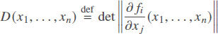
of the matrix of partial derivatives. Thus, the reversibility requirement means that this determinant should be constant: D(x₁,…,x_n) = const.

Reversibility of computing with real numbers: first case

Let us first consider the case when, in the original transformation, the number of outputs is the same as the number of inputs:

Of course, for many such real-life transformations – e.g. for a frequent transformation of all inputs into a log-scale (x₁, …,x_n) ↦ (ln(x₁),…, ln(x_n)) – the determinant D(x₁, …,x_n)is not a constant.

Since the original transformation of n inputs into n outputs is often not reversible, a reasonable idea is to add one or more auxiliary variables u₁,…,u_k, and to replace the original transformation with a new transformation

It turned out^[41] that this way, we can always turn the original transformation into a reversible one, and that for this, it is sufficient to add just one auxiliary variable u, i.e., to replace the original transformation with a new transformation

for an appropriate function v_f(^x₁,…,x_n, u).

Not only can we prove that there always exists an auxiliary function v_f(x₁,…, x_n, u) for which the new transformation is reversible, we can actually explicitly describe the corresponding auxiliary function. Indeed, as we have mentioned earlier, reversibility means that the determinant of the corresponding transformation should be equal to a constant c. One can show that the requirement that for the new transformation, the corresponding (n + 1)-dimensional determinant is equal to c, implies that

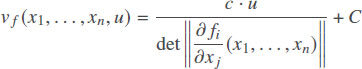
for some constant C. Vice versa, for thus defined auxiliary function v_f(x₁,…, x_n, u), the determinant is always equal to the constant c – and thus, the new transformation is indeed reversible.

Comment. The value of an additive constant C does not affect anything: we can always re-scale the auxiliary variable u into u’ = u – C and thus, make this constant equal to 0.

Reversibility of computing with real numbers: second case

What if the number of outputs is smaller than the number of inputs? In this case, we need to add additional outputs, to preserve reversibility. For example, a binary operation (x₁, x₂) ↦ f(x₁, x₂) has to be replaced with a transformation (x₁, x₂) ↦ (f (x₁, x₂), g(x₁, x₂)) for an appropriate auxiliary function g(x₁, x₂). The reversibility requirement – that the volume must be preserved – takes the form

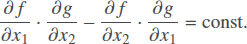
In this case, there is no general analytical expression for the solution, but there are explicit expressions for the usual binary operations f(x₁, x₂). For example, for addition f(x₁, x₂) = x₁ + x₂ one of the possible solutions is subtraction g(x₁, x₂) =x₁ – x₂; for multiplication f(x₁, x₂) = x₁ · x₂, we can take g(x₁, x₂) = ln(x₁/x₂), etc.

Comment. In this section, mathematics is much simpler than in the previous one, but still solving partial differential equations is not exactly trivial mathematics.

Physics vs. study of environment

The main difference between physics and study of environment is that:

• in physics, we usually have a theory that explains all – or at least almost all – observations, that predicts most important future events, while

• in the study of environment, no matter how complex we make our models, we are far from accurate predictions.

To some extent, the same is true in physics: theories change, they are updated. After Newton, most physicists were under the impression that Newtonian physics would be sufficient to explain all the world’s phenomena – and until the late 19th century, it was indeed mostly sufficient. However, new observations led to the need to replace Newtonian physics with more accurate relativistic and quantum approaches. Many physicists actually believe that in physics too, no matter what model we propose, no matter what law of nature we discover that fits all known observations, eventually a new observation will appear that will be inconsistent with this law – and thus, the law will need to be modified; see, e.g.,^[39,40]. In this section, we will describe the consequences of this widely spread belief.

How this belief affects computations

The above belief means, in particular, that the sequence of observations is not computable – if it was computable, i.e., if there existed an algorithm that predicts all observations, then this algorithm would not need any eventual modifications and would, thus, contradict this belief.

In other words, according to this belief, simply observing the world can help us come up with values that cannot come from any computations – i.e., observations have the ability beyond computations. Since observations have this beyond-usual-computations ability, it is reasonable to expect that using these observations in computations can speed up the computation process. This indeed turned out to be the case – although, similarly to the previous two sections, this conclusion requires some non-trivial mathematics.

To describe the exact result, we need to briefly recall several notions from theory of computation; for details, see, e.g. ^[23,43]. One of the main tasks of theory of computation is to distinguish between:

• feasible algorithms – i.e., algorithms that require reasonable computation time for inputs of reasonable length – and

• algorithms which require so much computation time that they are not practically possible: e.g., that require, for inputs of length 100, longer computation time than the lifetime of the Universe.

How to clearly separate feasible from non-feasible algorithms is still an open problem. At present, the best formalization – that, in most case, adequately describes feasibility – is to define an algorithm A to be feasible if there is a polynomial P(n) such that for each input of size n, this algorithm requires time bounded by P(n).

This condition can be describe as t_A (n) ≤ P(n), where t_A (n) is the largest computation time that the algorithm A needs to process inputs of size n. The dependence of t_A(n) on n is called the algorithms computational complexity. In these terms, the current definition identifies feasible algorithms with algorithms of no more than polynomial computational complexity.

(It should mentioned that this is not a perfect definition. For example, according to this definition, an algorithm that requires 10³⁰⁰ computational steps for each input – longer than the lifetime of the Universe – is called feasible, while an algorithm whose computational complexity grows as exp(10^–20 · n) is called infeasible. However, this definition is the best we have.)

The next natural question is which problems can be solved by feasible algorithms. To formalize this question, we need to formalize what is a problem. In most practical problems, while the problem itself may be difficult to solve, it is feasible to check whether a candidate for a solution is indeed a solution. For example:

• it is difficult to come up with a proof of a mathematical statement, but

• once someone gives us a text that is supposed to be a detailed proof, it is straightforward to check each step and confirm (or not) whether this is indeed a correct proof, with no unproven gaps.

The class of such problems – for which, once we have a candidate for a solution, we can feasibly check whether it is indeed a solution – is denoted by NP. For some of these problems, there is a feasible algorithm; the class of all such problems is denoted by P.

Whether all problems can be feasibly solved, i.e., whether P is equal to NP, is not known: this is a famous open problem. What is known is that in the class NP there are problems which are the most difficult in this class – in the sense that every other problem from the class NP can be feasible reduced to each of these problems. Such problems are known as NP-complete. Historically the first example of an NP-complete problem is the following propositional satisfiability (SAT) problem:

• given a propositional formula, i.e., an expression obtained from the Boolean (true-false) variables by using “and”, “or”, and “not”,

• find the values of these variables that make this formula true – or return a message that this formula is always false.

The paper^[44] studied what can be computed if we consider “physical” algorithms, i.e., algorithms, that, in addition to usual computational step, can access (and use) unrelated observations of the physical world. In this paper, it is proven that there exists a feasible physical algorithm A with the following property. For every ε > 0 and for every integer n, there exists a larger integer N > n for which the proportion of SAT formulas of length N that is correctly solved by this algorithm A is ≥ 1 – ε. In other words, if we use observations, then we can feasible solve most instances of hard problems. A similar result holds for all other NP-complete problems. So, under the assumption that the physicists’ belief is correct, observations indeed help computations.

Comment. The paper^[44] uses yet another area of non-trivial mathematics: the notions of meager sets, also known as sets of Baire first category; see, e.g.,^[45,46].

Why environment?

The above result is about observations in general: we can observe stars in the sky, we can observe how elementary particles interact in an accelerator, etc. So why are we citing this result in a paper about environment-related applications? The reason is simple: to get good results, we need a sufficiently large number of observations – observations that cannot be explained by simple formulas. We can get a lot of data by observing stars in the sky or planets, but their visible motion is well described by reasonably simple algorithms: already ancients could predict solar eclipses many years ahead.

Micro-world observations are not that easy to predict, but each observation requires a costly experiment, so we do not have that many data points. We have a lot of not-easy-to-predict data points from geological sciences, but much more data comes from observing environment: for environment-related data, we have the same spatial variability as for the geological data, but environmental data also has temporal variability, so instead of 2-D or 3-D data, we now have 3-D or 4-D data.

Environment learning and/or exploration can reduce the complexity of computational problems

Based on the general result from^[44] – that using physical observations can reduce the complexity of computational problems – and on the above argument that environment provided the largest number of not-easy-to-explain observations, we can conclude that observing environment can reduce (and reduce drastically) computation time needed to solve challenging computational problems. These observations can come either by simply observing the environment and learning from these observations – or from actively exploring the environment’s reaction to different actions.

The very fact that observing physical processes can speed up computations is well known. Many efficient algorithms simulate natural processes – genetic algorithms (and, more generally, evolutionary computations) simulate biological evolution, neural networks (in particular, deep neural networks) simulate how biological neurons process data, etc. In these two cases, observing biological evolution helped us to solve the problem of optimizing different objective functions, and observing how neuron-based brain learns new information helped solve the problem of designing machine learning tools. In general, if we have a complex computational problem, it makes sense to see if there is any natural phenomenon (e.g., environment-related one) which is similar to the problem that we are trying to solve, so that by observing this phenomenon, we can solve the corresponding problem.

That observations can help is a well-known fact. What was new in^[44] is a formal proof that this speed-up can be really drastic – in many cases, making the intractable problem, a problem which, in general, cannot be solved in feasible time – feasibly solvable.

What is Gaia hypothesis

As we have mentioned, the reason why we believe that environmental data can be helpful in computing is that this data is difficult to predict. But there is another known phenomenon which is also very difficult to predict – the behavior of human beings. In contrast to planets, we are not deterministic machines, we make choices, and these choices are difficult to predict. A natural idea is thus to conclude that the Earth is, in some reasonable sense, an intelligent being – similar to us. This, in a nutshell, is the main idea of the so-called Gaia hypothesis; see, e.g.,^[47].

At first glance, this hypothesis sounds like an unscientific mysticism; however, researchers made some sense of this hypothesis; see, e.g.,^[48-50]. What we propose is yet another rational interpretation of this hypothesis. Indeed, what is intelligence? It is largely the ability to solve complex problems – whether they are real-life complex problems or abstract ones. How do we know that someone has intelligence? Maybe we observe this person solving problems, maybe this person helps us solve complex problems.

From this viewpoint, since observing the environment can help us solve complex problems, we can therefore naturally say that in this sense, the Earth is an intelligent being – which is exactly what the Gaia hypothesis is claiming.

REFERENCES

1. Nielsen MA, Chuang IL. Quantum Computation and Quantum Information. Cambridge, UK: Cambridge University Press; 2000.
2. Starks SA, Kreinovich V. Environmentally-oriented processing of multi-spectral satellite images: new challenges for Bayesian methods. In: Erickson GJ, Rychert JT, Smith CR, editors. Maximum Entropy and Bayesian Methods Dordrecht: Kluwer; 1998. pp. 271-6.
3. Beck J. Data Processing under a Combination of Interval and Probabilistic Uncertainty and Its Application to Earth and Environmental Studies and Engineering.; 2004.
4. Kreinovich V, Longpré L, Starks SA, Xiang G, Beck J, Kandathi R, Nayak A, Ferson S, Hajagos J. Interval versions of statistical techniques, with applications to environmental analysis, bioinformatics, and privacy in statistical databases. Journal of Computational and Applied Mathematics 2007;199:418-23.
5. Jaimes A, Tweedie C, Magoč T, Kreinovich V, Ceberio M. Optimal sensor placement in environmental research: designing a sensor network under uncertainty. Proceedings of the 4th International Workshop on Reliable Engineering Computing REC’2010, Singapore, March 3-5, 2010:255-67.
6. Jaimes A, Tweedie C, Kreinovich V, Ceberio M. Scale-invariant approach to multi-criterion optimization under uncertainty, with applications to optimal sensor placement, in particular, to sensor placement in environmental research. International Journal of Reliability and Safety 2012;6:188-203.
7. Servin C, Ceberio M, Jaimes A, Tweedie C, Kreinovich V. How to describe and propagate uncertainty when processing time series: metrological and computational challenges, with potential applications to environmental studies In: Chen S-M, Pedrycz W, editors. Time Series Analysis, Modeling and Applications: A Computational Intelligence Perspective. Cham, Switzerland: Springer Verlag; 2013. pp. 279-99.
8. Brady J, Lerma O, Kreinovich V, Tweedie C. Toward computing an optimal trajectory for an environment-oriented Unmanned Aerial Vehicle (UAV) under uncertainty. Journal of Uncertain Systems 2015;9:84-94.
9. Kreinovich V, Ouncharoen R. Fuzzy (and interval) techniques in the age of big data: an overview with applications to environmental science, geosciences, engineering, and medicine. International Journal of Uncertainty, Fuzziness, and Knowledge-Based Systems 2015;23:75-89.
10. Escarzaga SM, Tweedie C, Kosheleva O, Kreinovich V. .
11. Escarzaga SM, Tweedie C, Kosheleva O, Kreinovich V. How to predict nesting sites and how to measure shoreline erosion: fuzzy and probabilistic techniques for environment-related spatial data processing. In: Zadeh L, Yager RR, Shahbazova SN, Reformat M, Kreinovich V, editors. Recent Developments and New Direction in Soft Computing: Foundations and Applications. Cham, Switzerland: Springer Verlag’; 2018. pp. 595-604.
12. Hilbert D. Mathematische Probleme. Nachrichten von der Königl. Gesellschaft der Wiss. zu Göttingen 1900;253–297; English translation: Mathematical Problems, lecture delivered before the International Congress of Mathematics in Paris in. 1900. translated in Bull. Amer. Math, Soc 1902;8:437-79. reprinted in Browder, FE, editor, Mathematical Developments Arising from Hilbert’s Problems. Providence, Rhode Island: American Math. Soc; 1976
13. Dehn M. Über raumgleiche Polyeder. Nachr. Acad. Wiss. Gottingen Math.-Phys. Kl 1900:345-54.
14. Dehn M. Über den Rauminhalt. Mathematische Annalen 1901;3:465-78.
15. Sydler JP. Conditions nécessaires et suffisantes pour l’équivalence des polyèdres de l’espace euclidean à trois dimensions. Comment Math Helv 1965;40:43-80.
16. Boltianskii VG. Hilbert’s Third Problem. Washington, D.C.: V. H. Winston & Sons; 1978.
17. Boltianskii VG. Combinatorial geometry. In: Gamrkrelidze RV, editor. Algebra, Topology, and Geometry Moscow: VINITI Publ; 1981. pp. 209-74. (in Russian)
18. Neumann WD. Hilbert’s 3rd problem and invariants of 3-manifolds. Geom Topol Monogr 1998;1:383-411.
19. Kellerhals R. Old and new on Hilbert’s third problem In: Proceedings of the 9th Meeting of European Women in Mathematics (EWM), Loccum, Germany, 1999. Cairo: Hindawi Pub.; 2000. pp. 179-87.
20. Benko D. A new approach to Hilbert’s third problem. American Mathematical Monthly 2007;114:665-76.
21. Kosheleva O, Kreinovich V. Geombinatorics, computational complexity, and saving environment: let’s start. Geombinatorics 1994;3:90-9.
22. Turing AM. On computable numbers, with an application to the Entscheidungsproblem. Proceedings of the London Mathematical Society 1936/37;42:230-65; A correction, ibid, 1937;43:544-46.
23. Kreinovich V, Lakeyev A, Rohn J, Kahl P. Computational Complexity and Feasibility of Data Processing and Interval Computations. Dordrecht: Kluwer; 1998.
24. Kosheleva OM. Axiomatization of volume in elementary geometry. Siberian Mathematical Journal 1980;21:106-114. (in Russian); English translation in Siberian Mathematical Journal 1980;21:78-85
25. Kosheleva O. Hilbert problems (almost) 100 years later (from the viewpoint of interval computations). Reliable Computing 1998;4:399-403.
26. Cooke DE, Duran R, Gates A, Kreinovich V. Geombinatoric problems of environmentally safe manufacturing and linear logic. Geombinatorics 1994;4:36-47.
27. Kreinovich V, Kosheleva O. An application of logic to combinatorial geometry: how many tetrahedra are equidecomposable with a cube? Mathematical Logic Quarterly 1994;40:31-34.
28. Courant R, Robbins H. Geometric constructions. The algebra of number fields. Ch. 3 in What Is Mathematics?: An Elementary Approach to Ideas and Methods. Oxford, England, UK: Oxford University Press; 1996. pp. 117-64.
29. Mohanty Y. Construction of a 3/4-ideal hyperbolic tetrahedron out of ideal tetrahedra. Discrete and Computational Geometry 2004;32:117-28.
30. Tarski A. A Decision Method for Elementary Algebra and Geometry. 2nd ed. Berkeley and Los Angeles; 1951. p. 63.
31. Basu S, Pollack R, Roy M-F. Algorithms in Real Algebraic Geometry. Berlin: Springer-Verlag; 2006.
32. Mishra B. Computational real algebraic geometry In: Handbook on Discreet and Computational Geometry. Boca Raton, Florida: CRC Press; 1997.
33. Kreinovich V. Equidecomposability (scissors congruence) of polyhedra in IR3 and IR4 is algorithmically decidable: Hilbert’s 3rd Problem revisited. Geombinatorics 2008;18:26-34.
34. Ge G. Algorithms Related to Multiplicative Representation of Algebraic Numbers.; 1993.
36. Babai L, Beals R, Cai J-Y, Ivanyos G, Luks EM. Multiplicative Equations Over Commuting Matrices, Princeton/Rutgers DIMACS Center. Technical Report, TR 95-32 1995.
37. Buchmann J, Eisenbrand F. On factor refinement in number fields. Mathematics Of Computation 1999;68:345-50.
38. Derksen H, Jeandel E, Koiran P. Quantum automata and algebraic groups. Journal of Symbolic Computation 2005;39:357-71.
39. Feynman R, Leighton R, Sands M. The Feynman Lectures on Physics. Boston, Massachusetts: Addison Wesley; 2005.
40. Thorne KS, Blandford RD. Modern Classical Physics: Optics, Fluids, Plasmas, Elasticity, Relativity, and Statistical Physics. Princeton, New Jersey: Princeton University Press; 2017.
41. O. Galindo, L. Bokati, V. Kreinovich. .
42. Galindo O, Kreinovich V. For quantum and reversible computing, intervals are more appropriate than general sets, and fuzzy numbers than general fuzzy sets. In: Proceedings of the Joint 11th Conference of the European Society for Fuzzy Logic and Technology EUSFLAT’2019 and International Quantum Systems Association (IQSA) Workshop on Quantum Structures, Prague, Czech Republic, September 9-13 2019; doi: 10.2991/eusflat-19.2019.89.
43. Papadimitriou C. Computational Complexity. Reading, Massachusetts: Addison Welsey; 1994.
44. Kosheleva O, Zakharevich M, Kreinovich V. If many physicists are right and no physical theory is perfect, then by using physical observations, we can feasibly solve almost all instances of each NP-complete problem. Mathematical Structures and Modeling 2014;31:4-17.
45. Jalal-Kamali A, Nebesky O, Durcholz MH, Kreinovich V, Longpré L. Towards a ‘generic notion of genericity: from ‘typical’ and ‘random’ to meager, shy, etc. Journal of Uncertain Systems 2012;6:104-13.
46. Oxtoby JC. Measure and Category: A Survey of the Analogies between Topological and Measure Spaces. New York, Heidelberg, Berlin: Springer Verlag; 1980.
47. Lovelock J. Gaia: A New Look at Life on Earth. Oxford, UK: Oxford University Press; 2000.
48. Lenton TM, Daines SJ, Dyke JG, Nicholson AE, Wilkinson DM, Williams HT. Selection for Gaia across multiple scales. Trends in Ecology & Evolution 2018;33:633-645.
49. Alcabes ODN, Olson S, Abbot DS. Robustness of Gaian feedbacks to climate perturbations. Monthly Notices of the Royal Astronomical Society 2020;492:2572-2577.
50. Vakulenko SA, Sudakov I, Petrovskii SV, Lukichev D. Stability of a planetary climate system with the biosphere competing for resources. Physics Reviews E 2021;103. Paper 022202
Cite This Article
Export citation file: BibTeX | RIS
OAE Style
Kreinovich V, Kosheleva O. Green computing: three examples of how non-trivial mathematical analysis can help. J Smart Environ Green Comput 2021;1:146-58. http://dx.doi.org/10.20517/jsegc.2021.11
AMA Style
Kreinovich V, Kosheleva O. Green computing: three examples of how non-trivial mathematical analysis can help. Journal of Smart Environments and Green Computing. 2021; 1(3): 146-58. http://dx.doi.org/10.20517/jsegc.2021.11
Chicago/Turabian Style
Kreinovich, Vladik, Olga Kosheleva. 2021. "Green computing: three examples of how non-trivial mathematical analysis can help" Journal of Smart Environments and Green Computing. 1, no.3: 146-58. http://dx.doi.org/10.20517/jsegc.2021.11
ACS Style
Kreinovich, V.; Kosheleva O. Green computing: three examples of how non-trivial mathematical analysis can help. . J. Smart. Environ. Green. Comput. 2021, 1, 146-58. http://dx.doi.org/10.20517/jsegc.2021.11
About This Article
Copyright
Data & Comments
Data
0
Cite This Article 2 clicks
Like This Article 10
likes
Comments
Comments must be written in English. Spam, offensive content, impersonation, and private information will not be permitted. If any comment is reported and identified as inappropriate content by OAE staff, the comment will be removed without notice. If you have any queries or need any help, please contact us at support@oaepublish.com.