Download PDF
Original Article  |  Open Access  |  29 Jun 2022

Adaptive multi-criteria group decision-making model based on consistency and consensus with intuitionistic reciprocal preference relations: a case study in energy storage technology selection

Views: 725 |  Downloads: 644 |  Cited:   8
J Smart Environ Green Comput 2022;2:58-75.
10.20517/jsegc.2022.15 |  © The Author(s) 2022.
Author Information
Article Notes
Cite This Article

Abstract

Aim: This study aims to present a multi-criteria group decision-making model with intuitionistic reciprocal preference relations that incorporates a new feedback mechanims adapting its operation to the decision-makers' consistency.

Methods: A new adaptive feedback mechanism is developed within a multi-criteria group decision-making model. Assuming different kinds of decision-makers classified according to their consistency, this feedback mechanism customizes the recommendations given by adopting three strategies to identify the problematic assessments that the decision-makers should change if they want to collaborate to increase the consensus.

Results: The performance of the proposed model is shown in a case study for the selection of an energy storage technology. It shows that the decision-makers providing assessments with low consistency must modify more assessments, allowing the most consistent decision-makers to be the leaders of the negotiation and persuade the others to adjust their assessments to improve the agreement achieved.

Conclusion: In this study, a novel multi-criteria group decision-making model is developed. It includes an adaptive feedback mechanism adjusting the advice provided by considering the decision-makers' consistency. It allows that the assessments of the most consistent decision-makers never be strongly modified during the decision process.

Keywords

Multi-criteria group decision-making, consensus, consistency, feedback mechanism, intuitionistic reciprocal preference relation, energy storage technology selection

INTRODUCTION

What way should I drive to work? What blouse or shirt to wear? Decision-making is a daily exercise done by human beings without hesitation, without thought. It is also a process and a habit with regard to organization, being the most critical process because successful and effective choices make a profit to the organization and failed ones make losses[1]. As a consequence, here, hesitation, fear and self doubt, may come.

The complicated nature of organizational environments makes hard to consider, for an individual decision-maker, all the features of a problem in order to make the choice. In addition, research suggests that groups make better decisions than individual decision-makers[2]. Many important decisions in society, such as governing bodies, committees, business partners, juries, and so on, are made by group of decision-makers[3].

Moving from an individual decision-maker to a group of them adds complexity to the decision-making process. For this reason, group decision-making models, such as voting-based models[4] or Delphi technique[5], among others, have been developed. The problem is now longer choosing the appropriate course of action or option among several alternative possibilities by considering an individual's opinion[6], but rather the study must be extended to consider the difference of opinion or level of dissatisfaction among several parties[7]. In consequence, consensus processes are usually carried out[8, 9].

Consensus is a process by which a group of decision-makers try to achieve an agreement. Here, the opinions of all participants are collected and integrated to arrive at a final decision acceptable to all, even if it is not the "favorite" of each decision-maker. That is, consensus requires that a majority accepts a given course of action, but that the minority approves to go along with the course of action[7]. To do it, the decision-makers must modify their initial opinions to align their positions.

Within the consensus process, a notable stage is the feedback mechanism[10], in which the decision-makers are advised to change their judgments to improve the agreement achieved. For this reason, a number of feedback mechanisms have been developed. In the first feedback mechanisms proposed[8, 11-13], the advice given to the decision-makers was provided by a person, called moderator. The shortcoming of these feedback mechanisms is the subjectivity that the moderator can introduce into the process. To avoid this subjectivity, automatic feedback mechanisms simulating the moderator's activity were developed[8, 14-17], making more efficient and effective the consensus process. Among them, those that adapt their operation to a given criterion, as, for example, the decision makers' knowledge[17] or the decision makers' credibility[14], have shown better performance[18]. However, the shortcoming of these approaches is that the values associated with the knowledge and the credibility are assigned subjectively. Therefore, it presents a similar problem that the approaches based on the moderator.

Given that feedback mechanisms are very relevant within the consensus process, this study aims to build a group decision-making model incorporating a new feedback mechanism that adapts its behaviour according to the decision-makers' consistency [19-21]. In particular, it adjusts the amount of advice required by each decision-maker depending on her/his consistency. Different from the existing adaptive feedback mechanisms, in this new one, the consistency related to each decision-maker is computed objectively instead of being assigned subjectively. This new feedback mechanism can also deal with decision-making problems in which the decision-makers use intuitionistic reciprocal preference relations (preference relations in which the pairwise comparisons are made via a membership degree and a non-membership degree) to express their assessments and it can manage multi-criteria contexts, i.e., decision-making problems in which different criteria are considered. Here, instead of assuming that the decision-makers provide their assessments between pairs of alternatives as a whole, different criteria are bare in mind[22]. For instance, let us suppose a project of renewable energy storage that, according to energy characteristics, energy demand, and local hydro geographic characteristics, considers different renewable energy storage technology alternatives, namely, Li-ion battery, supercapacitor, high temperature thermal energy storage and flywheels[23]. In a multi-criteria setting, the preference of an alternative over another one is evaluated according to different criteria such as storage capacity, input cost, emissions, economic benefit, response time, social acceptance, and so on.

The content of this study is divided into five sections. In Section "Background", we recall the basic concepts and procedures related to the proposed model. The new model for group decision-making is elaborated on in Section "A New Adaptive Multi-Criteria Group Decision-Making Model". Strong attention is given to the feedback mechanism. Section "Case Study: Selection of an energy Storage Technology" provides a case study that helps understand the performance of the proposed model. Finally, Section "Concluding Remarks" provides some concluding remarks about the advantages and disadvantages of the proposed model along with some further research directions.

BACKGROUND

This section recalls the definitions of the Atanassov's intuitionistic fuzzy sets and the intuitionistic reciprocal preference relations. Furthermore, a procedure to obtain the consistency associated with an intuitionistic reciprocal preference relation and a procedure to compute the agreement achieved between the assessments contained in a set of intuitionistic reciprocal preference relations are described.

Atanassov's intuitionistic fuzzy sets

As an extension of the concept of fuzzy set, Krassimir Atanassov introduced the notion of intuitionistic fuzzy set[24], which relaxes a fundamental assumption of the fuzzy set theory, i.e. the complement of a fuzzy set $$ B $$ has a membership function defined exclusively in regards to the membership function $$ \mu_{B}(y) $$ as $$ 1 - \mu_{B}(y) $$. Nevertheless, the Atanassov's intuitionistic fuzzy set theory assumes the referred sum rests on the condition of being equal or less than 1[24]. Concretely:

Definition 1[24] Let $$ A $$ be a non-empty universe. An Atanassov's intuitionistic fuzzy set (AIFS) $$ I $$ on $$ A $$ is defined as $$ I = \{(a, \mu_{I}(a), \nu_{I}(a)\; |\; a \in A\} $$ with $$ \mu_{I}(a) \in [0,1] $$ being the membership degree of the element $$ a $$ in $$ I $$ and $$ \nu_{I}(a) \in [0,1] $$ being the non-membership degree of the element $$ a $$ in $$ I $$, subject to the constraint $$ 0 \leq \mu_{I}(a) + \nu_{I}(a) \leq 1 $$.

On the one hand, the AIFS $$ I $$ becomes a fuzzy set whether, $$ \forall a \in A $$, $$ \mu_{I}(a) = 1 - \nu_{I}(a) $$. On the other hand, an additional criterion referred to as hesitancy index is needed whether at least a value $$ a \in A $$ fulfills $$ \mu_{I}(a) < 1 - \nu_{I}(a) $$. This hesitation index characterizes the amount of lacking of information in determining the membership degree of $$ a $$ to $$ I $$, being defined as $$ \tau_{I}(a) = 1 - \mu_{I}(a) - \nu_{I}(a) $$. The relationship between the membership degree and the non-membership degree, which is reciprocal, makes the second one needless because it can be determined from the first one in the case that $$ \tau_I(a) = 0 $$. The hesitancy index gives us an additional possibility of representing imperfect knowledge. This leads to describing many real problems in a more adequate way[25].

Intuitionistic reciprocal preference relations

As generalizations of the reciprocal preference relations, Zeshui Xu introduced the intuitionistic reciprocal preference relations[26]. They arise when AIFSs are used to make pairwise comparisons between the alternatives.

Definition 2[26] An intuitionistic reciprocal preference relation (IRPR) $$ R $$ on the set $$ A $$ is represented by a matrix $$ R = (r_{ij})_{n \times n} \subset A \times A $$ with $$ r_{ij} = \langle (a_i,a_j), \mu_R(a_i,a_j), \nu_R(a_i,a_j)\rangle $$$$ \forall i,j = 1,2,\dotsc,n $$. For convenience, let $$ r_{ij} = \langle \mu_{ij}, \nu_{ij}\rangle $$$$ \forall i,j = 1,2,\dotsc,n $$, where $$ r_{ij} $$ is an intuitionistic fuzzy value composed by the certainty degree $$ \mu_{ij} $$ to which $$ a_i $$ is preferred to $$ a_j $$ and the certainty degree $$ \nu_{ij} $$ to which $$ a_i $$ is non-preferred to $$ a_j $$, and $$ \pi_{ij} = 1 - \mu_{ij} - \nu_{ij} $$ is interpreted as the uncertainty degree to which $$ a_i $$ is preferred to $$ a_j $$. Furthermore, $$ \mu_{ij} $$ and $$ \nu_{ij} $$ satisfy the following conditions:

$$ \begin{align} 0 \leq \mu_{ij} + \nu_{ij} \leq 1 & \quad \forall i,j = 1,2,\dotsc,n \\ \mu_{ii} = \nu_{ii} = 0.5 & \quad \forall i = 1,2,\dotsc,n \\ \mu_{ji} = \nu_{ij} & \quad \forall i,j = 1,2,\dotsc,n \end{align} $$

Consistency

On the one hand, consistency is associated with the property of transitivity[27]. On the other hand, rationality is related to consistency[28]. The transitivity has been characterized in reciprocal preference relations in different ways. However, Chiclana et al.[29] proved most of them are incorrect and concluded that the multiplicative transitivity property is the most adequate. Formally, Wu and Chiclana[30] generalized this property to IRPR by, first, applying the extension principle[31] to the case in which, instead of crisp values in the unit interval, fuzzy sets are used as preference values. Second, they applied the representation theorem[32] to those fuzzy sets in order to obtain the property of multiplicative transitivity related to the fuzzy preference values. Third, they applied this result to the case when interval-valued fuzzy sets are used instead of fuzzy sets. It led to the extension of the property of multiplicative transitivity from reciprocal preference relations to interval-valued reciprocal preference relations. In the end, the property of multiplicative transitivity for IRPR was formulated by using the mathematical isomorphims between the AIFSs and the interval-valued fuzzy sets[33].

Definition 3[30] An IRPR $$ R $$ is multiplicative transitive if and only if:

$$ \begin{equation} \forall i,j,k : \begin{cases} \mu_{ij} \cdot \mu_{jk} \cdot \mu_{ki} = \mu_{ik} \cdot \mu_{kj} \cdot \mu_{ji}\\ (1 - \nu_{ij}) \cdot (1 - \nu_{jk}) \cdot (1 - \nu_{ki}) = (1 - \nu_{ik}) \cdot (1 - \nu_{kj}) \cdot (1 - \nu_{ji}) \end{cases} \end{equation} $$

Given two alternatives, $$ a_i $$ and $$ a_j $$, $$ i < j $$, its partially multiplicative transitivity based estimated intuitionistic preference value, $$ mr^{k}_{ij} = \langle mr^{k-}_{ij}, mr^{k+}_{ij}\rangle $$, may be calculated by means of other one $$ a_k $$, $$ k \neq i,j $$, and Equation (2), provided that the denominators are not zero, in the following way[30]:

$$ \begin{align} mr^{k-}_{ij} = \frac{\mu_{ik} \cdot \mu_{kj} \cdot \mu_{ji}}{\mu_{jk} \cdot \mu_{ki}} \qquad\qquad\qquad & mr^{k+}_{ij} = 1 - \frac{(1 - \nu_{ik}) \cdot (1 - \nu_{kj}) \cdot (1 - \nu_{ji})}{(1 - \nu_{jk}) \cdot (1 - \nu_{ki})} \end{align} $$

In Equation (2), both expressions are always true whether two of the three sub-indexes are equal. Let $$ i = k $$, $$ mr^{i+}_{ij} = \nu_{ij} $$ if $$ \nu_{ij} \neq 1 $$, and $$ mr^{i-}_{ij} = \mu_{ij} $$ if $$ \mu_{ij} \neq 0 $$. Due to $$ \nu_{ij} = \mu_{ji} $$, then $$ \nu_{ji} \neq 1 $$ if and only if $$ \mu_{ij} \neq 1 $$, and $$ \mu_{ji} \neq 0 $$ if and only if $$ \nu_{ij} \neq 0 $$. As a result, if $$ (r_{ij},r_{ji}) \neq (\langle 1,0\rangle, \langle 0,1\rangle) $$ and $$ i = k $$, then $$ r_{ij} = m^{i}_{ij} $$. In addition, if $$ (r_{ij},r_{ji}) \neq (\langle 0,1\rangle, \langle 1,0\rangle) $$ and $$ i = k $$, then $$ r_{ij} = m^{j}_{ij} $$. To be brief, we can compute the multiplicative transitivity based estimated intuitionistic preference value of a pair of alternatives, $$ a_i $$ and $$ a_j $$, if $$ (r_{ij},r_{ji}) \neq \{(\langle 1,0\rangle, \langle 0,1\rangle), (\langle 0,1\rangle, \langle 1,0\rangle)\} $$ and $$ k \in \{i,j\} $$. However, there not exists an indirect estimation process as described above. At last, assuming that $$ j = i $$, then $$ r_{ii} = \langle 0.5,0.5\rangle $$ by definition and $$ r_{ii} = mr^{k}_{ii} $$ whenever $$ r_{ik} \not\in (\langle 0,1\rangle, \langle 1,0 \rangle) $$.

The global multiplicative transitivity based estimated value related to a particular pair of alternatives, $$ a_i $$ and $$ a_j $$, is calculated as the mean of all their partially multiplicative transitivity based estimated values:

$$ \begin{align} mr^{-}_{ij} = \frac{\sum\limits_{k \in R^{01}_{ij}}{mr^{k-}_{ij}}}{\#R^{01}_{ij}} \qquad\qquad\qquad & mr^{+}_{ij} = \frac{\sum\limits_{k \in R^{01}_{ij}}{mr^{k+}_{ij}}}{\#R^{01}_{ij}} \end{align} $$

being $$ R^{01}_{ij} = \{k \neq i,j\; |\; (r_{ik}, r_{kj}) \not\in R^{01}\} $$, $$ R^{01} = \{(\langle 1,0\rangle, \langle 0,1\rangle), (\langle 0,1\rangle, \langle 1,0\rangle)\} $$, and $$ \#R^{01}_{ij} $$ the cardinality of $$ R^{01}_{ij} $$.

As a result of this, given an IRPR $$ R $$, the following multiplicative transitivity based IRPR, $$ MR = (\langle {mr}^{-}_{ij}, {mr}^{+}_{ij}\rangle) $$, may be computed[30]:

$$ \begin{align} mr^{-}_{ij} = \begin{cases} \frac{\sum\limits_{k \in R^{01}_{ij}}{mr^{k-}_{ij}}}{\#R^{01}_{ij}} &\quad i < j \\ 0.5 &\quad i = j \\ \frac{\sum\limits_{k \in R^{01}_{ji}}{mr^{k+}_{ji}}}{\#R^{01}_{ji}} &\quad i > j \end{cases} \qquad\qquad\qquad & mr^{+}_{ij} = \begin{cases} \frac{\sum\limits_{k \in R^{01}_{ij}}{mr^{k+}_{ij}}}{\#R^{01}_{ij}} &\quad i < j \\ 0.5 &\quad i = j \\ \frac{\sum\limits_{k \in R^{01}_{ji}}{mr^{k-}_{ji}}}{\#R^{01}_{ji}} &\quad i > j \end{cases} \end{align} $$

If an IRPR $$ R $$ is multiplicative transitive then $$ R = MR $$. Certainly, if $$ R $$ is multiplicative transitive both expressions in Equation (2) are true $$ \forall i, j, k $$. That is:

$$ \begin{align} \mu_{ij} = \frac{\mu_{ik} \cdot \mu_{kj} \cdot \mu_{ji}}{\mu_{jk} \cdot \mu_{ki}} \qquad\qquad\qquad & \nu_{ij} = 1 - \frac{(1 - \nu_{ik}) \cdot (1 - \nu_{kj}) \cdot (1 - \nu_{ji})}{(1 - \nu_{jk}) \cdot (1 - \nu_{ki})} \end{align} $$

whenever $$ k \in R^{01}_{ij} $$. As a result of this, $$ mr^{k+}_{ij} = \nu_{ij} $$ and $$ mr^{k-}_{ij} = \mu_{ij} $$, $$ \forall i,j,k \in R^{01}_{ij} $$, proving that $$ r_{ij} = mr_{ij} $$, $$ \forall i,j $$. An IRPR $$ R $$ is referred to as multiplicative consistent if $$ R = MR $$[30].

Based on these results, a procedure to compute the consistency level, called $$ cl $$, of an IRPR $$ R $$ was built[30], which is based on the similarity between $$ R $$ and its multiplicative transitivity based IRPR, $$ MR $$, that is used to compute a consistency measure, $$ cl_{ij} $$, related to a pair of alternatives, $$ a_i $$ and $$ a_j $$, and a consistency measure, $$ cl_i $$, related to an alternative $$ a_i $$. These two consistency measures are used to compute the consistency level $$ cl $$. It is as follows:

$$ \begin{align} cl_{ij} = &\; 1 - d(r_{ij}, mr_{ij}) \end{align} $$

$$ \begin{align} cl_i =&\; \frac{\sum^{n}_{j=1;\; i \neq j}{cl_{ij}}}{n-1} \end{align} $$

$$ \begin{align} cl = &\; \frac{\sum^{n}_{i = 1}{cl_i}}{n} \end{align} $$

being $$ d $$ a metric describing the distance between two AIFSs that is used to define a similarity function between two AIFSs[34].

Consensus

Cabrerizo et al.[35] introduced a procedure to measure the consensus, called $$ cr $$, achieved between the decision-makers that participate in a multi-criteria group decision-making problem when they use IRPRs to provide their assessments. This procedure is based on the coincidence concept[36], which has been used in many approaches measuring the consensus in group decision-making problems. Assuming a group of $$ m $$ decision-makers, $$ DM = \{dm_1,dm_2,\dotsc,dm_m\} $$, a collection of $$ n $$ alternatives, $$ A = \{a_1,a_2,\dotsc,a_n\} $$, and a set of $$ q $$ criteria, $$ C = \{c_1,c_2,\dotsc,c_q\} $$, which have associated a importance weight $$ w_l \in [0,1] $$ such that $$ \sum_{l = 1}^{q}{w_l} = 1 $$, then the description of the procedure to obtain the consensus is the following:

● Calculation of a matrix for each pair of decision-makers, $$ dm_g $$ and $$ dm_h $$ ($$ g \neq h $$), and each criterion, $$ c_l $$, denoted as $$ SM^{ghl} = (sm^{ghl}_{ij}) $$, characterizing the similarity between the IRPRs $$ R^{gl} $$ and $$ R^{hl} $$ given by these decision-makers taking into account that criterion:

$$ \begin{equation} sm^{ghl}_{ij} = 1 - d(r^{gl}_{ij},r^{hl}_{ij}) \end{equation} $$

being $$ d $$ a metric that determines the distance between two AIFSs[34].

● Calculation of a matrix for each criterion, $$ c_l $$, denoted as $$ CM^l = (cm^{l}_{ij}) $$, characterizing the agreement achieved by the decision-makers on the criterion $$ c_l $$:

$$ cm_{ij}^l = \frac{2}{{m \cdot (m - 1)}}\sum\limits_{g = 1}^{m - 1} {\sum\limits_{h = g + 1}^m {sm_{ij}^{ghl}} } $$

● Calculation, for each matrix $$ CM^l $$, of three consensus measures, namely, a measure of consensus, $$ cp^{l}_{ij} $$, related to a pair of alternatives, $$ a_i $$ and $$ a_j $$, a measure of consensus, $$ ca^{l}_{i} $$, related to an alternative, $$ a_i $$, and a measure of global consensus, $$ cr^l $$. They are calculated as:

$$ \begin{align} cp^l_{ij} = &\; cm^l_{ij} \end{align} $$

$$ \begin{align} ca^l_i = &\; \frac{\sum^{n}_{j = 1; j \neq i}{cp^l_{ij}}}{n-1} \end{align} $$

$$ \begin{align} cr^l = &\; \frac{\sum^n_{i=1}{ca^l_i}}{n} \end{align} $$

● Calculation of $$ cr $$ by means of the weighted mean of the $$ cr^l $$:

$$ cr = \sum\limits_{l = 1}^q {{w_l} \cdot c{r^l}} $$

A NEW ADAPTIVE MULTI-CRITERIA GROUP DECISION-MAKING MODEL

We present a new adaptive group decision-making method that deal with multi-criteria contexts in which the decision-makers make use of IRPRs to express their assessments. It is structured in the following five stages (see Figure 1): (i) articulation of the IRPRs; (ii) analysis of consensus; (iii) feedback mechanism; (iv) calculation of the collective IRPR; and (v) ranking of the alternatives. Its main novelty is that it incorporates a feedback mechanism that is able to deal with multi-criteria settings and it is based on the decision-makers' consistency in such a way that it provides more recommendations to the decision-makers with lower consistency levels than to the decision-makers with higher consistency levels. Next, we elaborate on the above stages in detail.

Adaptive multi-criteria group decision-making model based on consistency and consensus with intuitionistic reciprocal preference relations: a case study in energy storage technology selection

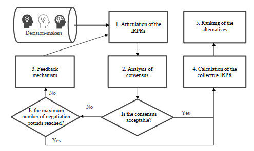
Figure 1. Graphical scheme of the proposed model.

Articulation of the IRPRs

The starting point is a group of $$ m $$ decision-makers, $$ DM = \{dm_1,dm_2,\dotsc,dm_m\} $$, a collection of $$ n $$ alternatives, $$ A = \{a_1,a_2,\dotsc,a_n\} $$, and a set of $$ q $$ criteria, $$ C = \{c_1,c_2,\dotsc,c_q\} $$, that are born in mind to evaluate the alternatives. In addition, every criterion $$ c_l \in C $$ has associated a importance weight $$ w_l \in [0,1] $$ such that $$ \sum_{l = 1}^{q}{w_l} = 1 $$. Here, IRPRs are assumed to model the comparisons between alternatives given by the decision-makers because the use of AIFSs allows an additional freedom degree modeling hesitancy of individuals related to the exclusion and inclusion of an element to a set[25]. Therefore, once the decision-makers have expressed their assessments, we get a set of $$ m \cdot q $$ IRPRs, $$ R^{gl} $$, $$ g = 1,\dotsc, m $$, $$ l = 1,\dotsc,q $$, of dimension $$ n \times n $$.

Analysis of consensus

The second stage consists in analyzing the consensus achieved. When all the decision-makers have given their IRPRs, the procedure described in Section Background is carried out to measure the consensus achieved. Concretely, the value of $$ cr $$ determines the consensus achieved. Usually, a consensus threshold, $$ \alpha \in [0,1] $$, which is conditioned by the given decision-making problem[15], is compared with the value of $$ cr $$. The next stage, i.e. the feedback mechanism, is executed with the objective of supporting decision-makers in modifying their assessments to increase the consensus achieved if $$ \alpha $$ is greater than $$ cr $$. If not, the fourth stage, i.e. the calculation of the collective IRPR, is conducted. Furthermore, as a mean to avoid a state in which the consensus reached does not converge to the consensus threshold, the negotiation rounds are limited to a maximum number that is decided at the beginning of the decision-making process[15]. As a consequence, the fourth stage is also executed if the current negotiation round exceeds the maximum number of negotiation rounds.

Feedback mechanism

We introduce a new feedback mechanism assuming that decision-makers with lower consistency levels need more advice than those with higher consistency levels. That is, because a low consistency level means that the decision-maker has provided contradictory assessments, it seems logical that the decision-makers providing inconsistency assessments will require more advice on how to modify their judgments. If a decision-maker has expressed contradictory assessments, it could mean that she or he does not have the enough level of knowledge about the alternatives and the criteria. Therefore, more adjustments in their assessments should be needed to lead a consensual decision. On the contrary, decision-makers with higher consistency levels will need low adjustments in their assessments to lead to consensus. Based on this assumption, this new feedback mechanism adapts its operation according to the decision-makers' consistency. This feedback mechanism, composed of four stages: (i) classifying of the decision-makers; (ii)computing proximity measures; (iii) looking for problematic assessments; and (iv) giving advice, is presented in what follows.

Classifying of the decision-makers

This task is accomplished by including each decision-maker into one of these subsets according to her or his consistency level: (i) very consistent, $$ DM_{vc} $$; (ii) consistent, $$ DM_{c} $$; and (iii) hardly consistent, $$ DM_{hd} $$. The consistency level is understood as a fuzzy subset with a membership function. In such manner, $$ cl^g \in [0,1] $$ denotes the consistency level of the decision-maker $$ dm_g $$. Then, a fuzzy matching mechanism, whose parameters depend on the problem at hand, is applied to done this classification. Each subset of decision-makers is a fuzzy set characterized by a membership function and two membership thresholds, $$ \beta_1 $$ and $$ \beta_2 $$, are established to differentiate the subsets. For a given decision-maker, $$ dm_g $$, her or his consistency level, $$ cl^g $$, is computed as:

$$ \begin{equation} cl^g = \sum\limits_{l = 1}^{q}{w_l \cdot cl^{gl}} \end{equation} $$

being $$ cl^{gl} $$ the consistency level associated with the IRPR $$ R^{gl} $$ provided by the decision-maker $$ dm_g $$ on the criterion $$ c_l $$, which is computed as described in Section Background.

Computing proximity measures

Once the decision-makers have been classified into one of the subsets, some proximity measures, which compute the agreement level between the individual IRPRs given by the decision-makers and the group one, are computed. This is done as follows[8]:

● Computation of a collective IRPR, $$ S^{l} = (s^{l}_{ij}) $$, for each criterion $$ c_l $$, by means of the aggregation of all the individual IRPRs given by the decision makers on that criterion:

$$ \begin{equation} s^{l}_{ij}= \frac{\sum^{m}_{g=1}{cl^{gl}} \cdot r^{gl}_{ij}}{\sum^{m}_{g=1}{cl^{gl}}} \end{equation} $$

In the aggregation, we must bear in mind that the decision-makers have distinct consistency levels that can act as weights of the aggregation. This is done by transforming the intuitionistic fuzzy value under the weight to generate a new value[37], which is used in the aggregation. In Equation (17), this is done by means of the weighted average.

● Once the collective IRPRs have been calculated, three proximity measures, namely, a measure of proximity, $$ pp^{gl}_{ij} $$, related to a pair of alternatives, $$ a_i $$ and $$ a_j $$, a measure of proximity, $$ pa^{gl}_{i} $$, related to an alternative, $$ a_i $$, and a measure of proximity on the relation, $$ pr^{gl} $$, are computed for each decision-maker, $$ dm^g $$, in each criterion, $$ c_l $$, as:

$$ \begin{align} pp^{gl}_{ij} = &\; 1- d(r^{gl}_{ij}, s^{l}_{ij}) \end{align} $$

$$ \begin{align} pa^{gl}_{i} = &\; \frac{\sum^{n}_{j=1, j \neq i}{pp^{gl}_{ij}}}{n-1} \end{align} $$

$$ \begin{align} pr^{gl} = &\; \frac{\sum^{n}_{i=1}{pa^{gl}_{i}}}{n} \end{align} $$

being $$ d $$ a metric that determines the distance between two AIFSs[34].

For each criterion, these three measures of proximity obtain the similarity between the assessment provided by the decision-maker and the collective one on a pair of alternatives, the similarity between the assessments provided by the decision-maker on an alternative and the collective one, and the similarity between the IRPR provided by the decision-maker and the collective one, respectively.

Looking for problematic assessments

This task consists in determining the problematic assessments, that is, those that should be adjusted to improve the consensus in the next round of negotiation. To identify these assessments, three strategies are applied according to the subset in which the decision-maker is included.

1. Determining problematic assessments for hardly consistent decision-makers. According to the common sense, the decision-makers included in this subset give less knowledgeable assessments. Consequently, more modifications are needed here. Hence, in this subset, we apply an strategy trying to adjust the assessments on all pair of alternatives having a low agreement. It is carried out as follows:

(a) Determining the pairs of alternatives, $$ PA^l_{hc} $$, for each criterion $$ c_l $$ whose measure of consensus is lower than $$ cr^l $$, which acts as an threshold:

$$ \begin{equation} PA^l_{hc} = \{(a_i,a_j)\ |\ cp^{l}_{ij}< cr^l \} \end{equation} $$

(b) Determining the problematic assessments, $$ PAS^{l}_{hc} $$, for each criterion $$ c_l $$, that each decision-maker $$ dm^{g}\in DM_{hc} $$ should modify:

$$ \begin{equation} PAS^{l}_{hc}= PA^l_{hc} \end{equation} $$

2. Determining problematic assessments for consistent decision-makers. This strategy tries to reduce the number of changes suggested to the decision-makers. This is done by analyzing the agreement from the viewpoint of the alternatives, that is, it only takes into account the assessments of the alternatives in which the agreement is not enough, rather than focusing on all the pairs of alternatives. Furthermore, different from the previous strategy, in which all the decision-makers are required to adjust the determined assessments, here, only the decision-makers whose measure of proximity at the level of alternatives is lower than a threshold are required to modify their assessments. It is carried out as follows:

(a) Determining the alternatives, $$ A^l_{c} $$, for each criterion $$ c_l $$ to be adjusted:

$$ \begin{equation} A^l_{c} = \{a_i\ |\ ca^l_{i} < cr^l \} \end{equation} $$

(b) Determining the pairs of alternatives, $$ PA^l_{c} $$, for each criterion $$ c_l $$ to be adjusted:

$$ \begin{equation} PA^l_{c} = \{(a_i,a_j)\ |\ a_i \in A^l_c \wedge cp^l_{ij} < cr^l \}\ \end{equation} $$

(c) Determining a threshold, $$ \gamma^{l}_{i} $$, for each alternative $$ a_i \in A^l_c $$, as follows:

$$ \gamma _i^l = \frac{1}{m}\sum\limits_{g = 1}^m p a_i^{gl} $$

(d) Determining the problematic assessments, $$ PAS^{l}_{c} $$, for each criterion $$ c_l $$, that each decision-maker $$ dm^{g}\in DM_{c} $$ should change:

$$ \begin{equation} PAS^{l}_{c}= \{(a_i,a_j) \in PA^l_c\ |\ pa^{gl}_{i}< \gamma^l_{i} \} \end{equation} $$

3. Determining problematic assessments for very consistent decision-makers. Here, we deal with the decision-makers included in $$ DM_{vc} $$, i.e. the decision-makers whose consistency is so high that they do not required many adjustments in their assessments to get a well-considered assessments. As a result, fewer adjustments than in the previous two strategies must be proposed. Particularly, for the pairs of alternatives determined in disagreement, it only adjusts the decision-makers' assessments whose measure of proximity is lower than a threshold at the level of pair of alternatives. It is carried out as follows:

(a) Determining the alternatives, $$ A^l_{vc} $$, for each criterion $$ c_l $$ to be adjusted:

$$ \begin{equation} A^l_{vc} = \{a_i\ |\ ca^l_{i} < cr_l \}\ \end{equation} $$

(b) Determining the pairs of alternatives, $$ PA^l_{vc} $$, for each criterion $$ c_l $$ to be adjusted:

$$ \begin{equation} PA^l_{vc} = \{(a_i,a_j)\ |\ a_i \in A^l_{vc} \wedge cp^{l}_{ij}< cr_l \}\ \end{equation} $$

(c) A threshold $$ \delta^{l}_{ij} $$, for each pair of alternatives $$ (a_i,a_j) \in PA^l_{vc} $$, is determined as follows:

$$ \delta _{ij}^l = \frac{1}{m}\sum\limits_{g = 1}^m p p_{ij}^{gl} $$

(d) Determining the problematic assessments, $$ PAS^{l}_{vc} $$, for each criterion $$ c_l $$, that each decision-maker $$ dm^{g}\in DM_{vc} $$ should change:

$$ \begin{equation} PAS^{l}_{vc}= \{(a_i,a_j) \in PA^l_{vc}\ |\ pa^{gl}_{i} < \gamma^{l}_{i} \wedge pp^{gl}_{ij} < \delta^{l}_{ij} \} \end{equation} $$

Giving advice

Once the problematic assessments have been recognized, the decision-makers need advice on how to modify their assessments. Concretely, for each assessment recognized as problematic, its adjustment is suggested by the feedback mechanism as follows:

● If $$ r^{gl}_{ij} > s^{l}_{ij} $$, the assessment expressed by the decision-maker $$ dm_g $$ on the pair $$ a_i $$ and $$ a_j $$ must be decreased.

● If $$ r^{gl}_{ij} < s^{l}_{ij} $$, the assessment expressed by the decision-maker $$ dm_g $$ on the pair $$ a_i $$ and $$ a_j $$ must be increased.

Calculation of the collective IRPR

The collective IRPR is computed by fusing all the individual decision-makers' IRPRs, which is performed by using a given aggregation function[38]. In this study, because we take into account a number of criteria and weights of importance associated with them, the weighted arithmetic mean is applied as aggregation function. Concretely, the collective IRPR is obtaining by means of the following procedure:

● A collective IRPR, $$ S^{l} = (s^{l}_{ij}) $$, is computed for each criterion $$ c_l $$ by means of Equation (17).

● Using the information contained in the collective IRPRs related to the criteria, the collective IRPR, $$ S = (s_{ij}) $$, is calculated as follows:

$$ \begin{equation} s_{ij} = \sum\limits_{l = 1}^{q}{w_{l} \cdot s^{l}_{ij}} \end{equation} $$

Ranking of the alternatives

To rank the alternatives solving the multi-criteria decision-making problem from best to worst, the information contained in the collective IRPR must be exploited. Distinct functions could be applied to perform this task[39]. Among them, we use the quantifier-guided dominance degree, $$ QGDD_i $$, that is computed as follows:

$$ \begin{equation} QGDD_i = \frac{1}{n-1}\sum\limits_{j = 1; j\neq i}^{n}{s_{ij}} \end{equation} $$

This choice degree of alternatives determines the dominance that the alternative $$ a_i $$ has over the remaining alternatives. The higher the value of $$ QGDD_i $$, the best the alternative $$ a_i $$ as solution to the decision-making problem.

CASE STUDY: SELECTION OF AN ENERGY STORAGE TECHNOLOGY

For a project of renewable energy storage, a number of possible alternatives of renewable energy storage technologies are selected according to energy characteristics, energy demand, local hydro geographic characteristics, and so on. These alternatives are: (i) Li-ion battery ($$ a_1 $$); (ii) supercapacitor ($$ a_2 $$); (iii) high temperature thermal energy storage ($$ a_3) $$; and (iv) flywheels ($$ a_4 $$). To select the best technology, four decision-makers, $$ dm_1 $$, $$ dm_2 $$, $$ dm_3 $$ and $$ dm_4 $$, who are expert in related fields, are bring together. They have to provide their assessments according to three criteria: (i) Storage capacity ($$ c_1 $$); (ii) input cost ($$ c_2 $$); and (iii) social acceptance ($$ c_3 $$). The importance weights of these criteria are $$ w_1 = 0.2 $$, $$ w_2 = 0.3 $$, and $$ w_3 = 0.5 $$.

In what follows, we illustrate the application of the proposed model to solve this multi-criteria group decision-making problem. In the first negotiation round (we assume a maximum number of five rounds), all the stages are described in detail. However, in the following negotiation rounds, only the most relevant information is provided, namely, the IRPRs given by the decision-makers, the consensus achieved and the advice provided by the feedback mechanism.

First negotiation round

Articulation of the IRPRs

The assessments, in the form of IRPRs, provided initially by the decision-makers are:

$$ R^{11}= \begin{bmatrix} \langle 0.50, 0.50 \rangle & \langle 0.70, 0.30 \rangle & \langle 0.60, 0.40 \rangle & \langle 0.30, 0.70 \rangle\\ \langle 0.30, 0.70 \rangle & \langle 0.50, 0.50 \rangle & \langle 0.50, 0.40 \rangle & \langle 0.30, 0.70 \rangle\\ \langle 0.40, 0.60 \rangle & \langle 0.40, 0.50 \rangle & \langle 0.50, 0.50 \rangle & \langle 0.60, 0.40 \rangle\\ \langle 0.70, 0.30 \rangle & \langle 0.70, 0.30 \rangle & \langle 0.40, 0.60 \rangle & \langle 0.50, 0.50 \rangle \end{bmatrix} \quad R^{12} = \begin{bmatrix} \langle 0.50, 0.50 \rangle & \langle 0.70, 0.20 \rangle & \langle 0.70, 0.30 \rangle & \langle 0.20, 0.70 \rangle\\ \langle 0.20, 0.70 \rangle & \langle 0.50, 0.50 \rangle & \langle 0.70, 0.20 \rangle & \langle 0.20, 0.70 \rangle\\ \langle 0.30, 0.70 \rangle & \langle 0.20, 0.70 \rangle & \langle 0.50, 0.50 \rangle & \langle 0.40, 0.60 \rangle\\ \langle 0.70, 0.20 \rangle & \langle 0.70, 0.20 \rangle & \langle 0.60, 0.40 \rangle & \langle 0.50, 0.50 \rangle \end{bmatrix} $$

$$ R^{13} = \begin{bmatrix} \langle 0.50, 0.50 \rangle & \langle 0.50, 0.50 \rangle & \langle 0.50, 0.50 \rangle & \langle 0.50, 0.50 \rangle\\ \langle 0.50, 0.50 \rangle & \langle 0.50, 0.50 \rangle & \langle 0.30, 0.70 \rangle & \langle 0.60, 0.30 \rangle\\ \langle 0.50, 0.50 \rangle & \langle 0.70, 0.30 \rangle & \langle 0.50, 0.50 \rangle & \langle 0.20, 0.70 \rangle\\ \langle 0.50, 0.50 \rangle & \langle 0.30, 0.60 \rangle & \langle 0.70, 0.20 \rangle & \langle 0.50, 0.50 \rangle \end{bmatrix} \quad R^{21} = \begin{bmatrix} \langle 0.50, 0.50 \rangle & \langle 0.20, 0.70 \rangle & \langle 0.70, 0.30 \rangle & \langle 0.60, 0.30 \rangle\\ \langle 0.70, 0.20 \rangle & \langle 0.50, 0.50 \rangle & \langle 0.90, 0.10 \rangle & \langle 0.30, 0.60 \rangle\\ \langle 0.30, 0.70 \rangle & \langle 0.10, 0.90 \rangle & \langle 0.50, 0.50 \rangle & \langle 0.60, 0.40 \rangle\\ \langle 0.30, 0.60 \rangle & \langle 0.60, 0.30 \rangle & \langle 0.40, 0.60 \rangle & \langle 0.50, 0.50 \rangle \end{bmatrix} $$

$$ R^{22} = \begin{bmatrix} \langle 0.50, 0.50 \rangle & \langle 0.50, 0.50 \rangle & \langle 0.30, 0.70 \rangle & \langle 0.50, 0.50 \rangle\\ \langle 0.50, 0.50 \rangle & \langle 0.50, 0.50 \rangle & \langle 0.80, 0.10 \rangle & \langle 0.70, 0.30 \rangle\\ \langle 0.70, 0.30 \rangle & \langle 0.10, 0.80 \rangle & \langle 0.50, 0.50 \rangle & \langle 0.20, 0.70 \rangle\\ \langle 0.50, 0.50 \rangle & \langle 0.30, 0.70 \rangle & \langle 0.70, 0.20 \rangle & \langle 0.50, 0.50 \rangle \end{bmatrix} \quad R^{23} = \begin{bmatrix} \langle 0.50, 0.50 \rangle & \langle 0.20, 0.80 \rangle & \langle 0.70, 0.20 \rangle & \langle 0.60, 0.40 \rangle\\ \langle 0.80, 0.20 \rangle & \langle 0.50, 0.50 \rangle & \langle 0.70, 0.20 \rangle & \langle 0.70, 0.30 \rangle\\ \langle 0.20, 0.70 \rangle & \langle 0.20, 0.70 \rangle & \langle 0.50, 0.50 \rangle & \langle 0.60, 0.40 \rangle\\ \langle 0.40, 0.60 \rangle & \langle 0.30, 0.70 \rangle & \langle 0.40, 0.60 \rangle & \langle 0.50, 0.50 \rangle \end{bmatrix} $$

$$ R^{31} = \begin{bmatrix} \langle 0.50, 0.50 \rangle & \langle 0.70, 0.20 \rangle & \langle 0.60, 0.40 \rangle & \langle 0.30, 0.70 \rangle\\ \langle 0.20, 0.70 \rangle & \langle 0.50, 0.50 \rangle & \langle 0.60, 0.30 \rangle & \langle 0.80, 0.10 \rangle\\ \langle 0.40, 0.60 \rangle & \langle 0.30, 0.60 \rangle & \langle 0.50, 0.50 \rangle & \langle 0.90, 0.10 \rangle\\ \langle 0.70, 0.30 \rangle & \langle 0.10, 0.80 \rangle & \langle 0.10, 0.90 \rangle & \langle 0.50, 0.50 \rangle \end{bmatrix} \quad R^{32} = \begin{bmatrix} \langle 0.50, 0.50 \rangle & \langle 0.40, 0.60 \rangle & \langle 0.40, 0.60 \rangle & \langle 0.20, 0.80 \rangle\\ \langle 0.60, 0.40 \rangle & \langle 0.50, 0.50 \rangle & \langle 0.50, 0.50 \rangle & \langle 0.80, 0.20 \rangle\\ \langle 0.60, 0.40 \rangle & \langle 0.50, 0.50 \rangle & \langle 0.50, 0.50 \rangle & \langle 0.20, 0.70 \rangle\\ \langle 0.80, 0.20 \rangle & \langle 0.20, 0.80 \rangle & \langle 0.70, 0.20 \rangle & \langle 0.50, 0.50 \rangle \end{bmatrix} $$

$$ R^{33} = \begin{bmatrix} \langle 0.50, 0.50 \rangle & \langle 0.80, 0.20 \rangle & \langle 0.20, 0.80 \rangle & \langle 0.20, 0.70 \rangle\\ \langle 0.20, 0.80 \rangle & \langle 0.50, 0.50 \rangle & \langle 0.40, 0.60 \rangle & \langle 0.50, 0.50 \rangle\\ \langle 0.80, 0.20 \rangle & \langle 0.60, 0.40 \rangle & \langle 0.50, 0.50 \rangle & \langle 0.70, 0.20 \rangle\\ \langle 0.70, 0.20 \rangle & \langle 0.50, 0.50 \rangle & \langle 0.20, 0.70 \rangle & \langle 0.50, 0.50 \rangle \end{bmatrix} \quad R^{41} = \begin{bmatrix} \langle 0.50, 0.50 \rangle & \langle 0.80, 0.10 \rangle & \langle 0.20, 0.70 \rangle & \langle 0.60, 0.30 \rangle\\ \langle 0.10, 0.80 \rangle & \langle 0.50, 0.50 \rangle & \langle 0.60, 0.40 \rangle & \langle 0.20, 0.70 \rangle\\ \langle 0.70, 0.20 \rangle & \langle 0.40, 0.60 \rangle & \langle 0.50, 0.50 \rangle & \langle 0.60, 0.40 \rangle\\ \langle 0.30, 0.60 \rangle & \langle 0.70, 0.20 \rangle & \langle 0.40, 0.60 \rangle & \langle 0.50, 0.50 \rangle \end{bmatrix} $$

$$ R^{42} = \begin{bmatrix} \langle 0.50, 0.50 \rangle & \langle 0.70, 0.30 \rangle & \langle 0.50, 0.50 \rangle & \langle 0.70, 0.30 \rangle\\ \langle 0.30, 0.70 \rangle & \langle 0.50, 0.50 \rangle & \langle 0.40, 0.60 \rangle & \langle 0.70, 0.20 \rangle\\ \langle 0.50, 0.50 \rangle & \langle 0.60, 0.40 \rangle & \langle 0.50, 0.50 \rangle & \langle 0.50, 0.50 \rangle\\ \langle 0.30, 0.70 \rangle & \langle 0.20, 0.70 \rangle & \langle 0.50, 0.50 \rangle & \langle 0.50, 0.50 \rangle \end{bmatrix} \quad R^{43} = \begin{bmatrix} \langle 0.50, 0.50 \rangle & \langle 0.70, 0.30 \rangle & \langle 0.10, 0.90 \rangle & \langle 0.10, 0.90 \rangle\\ \langle 0.30, 0.70 \rangle & \langle 0.50, 0.50 \rangle & \langle 0.20, 0.70 \rangle & \langle 0.20, 0.70 \rangle\\ \langle 0.90, 0.10 \rangle & \langle 0.70, 0.20 \rangle & \langle 0.50, 0.50 \rangle & \langle 0.30, 0.70 \rangle\\ \langle 0.90, 0.10 \rangle & \langle 0.70, 0.20 \rangle & \langle 0.70, 0.30 \rangle & \langle 0.50, 0.50 \rangle \end{bmatrix} $$

Analysis of consensus

To analyse the consensus achieved, the procedure described in Section "Background" is applied, using the Hamming distance between two AIFSs, $$ I_1 $$ and $$ I_2 $$, as $$ d $$ in Equation (10), however, other distance metrics of AIFSs could be used [34]. This distance is defined as [34]:

$$ \begin{equation} d(I_1,I_2) = \frac{1}{2}\sum\limits_{i = 1}^{n}{[| \mu_{I_1}(a_i) - \mu_{I_2}(a_i) | + | \nu_{I_1}(a_i) - \nu_{I_2}(a_i) |]} \end{equation} $$

First, the similarity matrices for each pair of decision-makers, which are omitted, are calculated. Then, a consensus matrix $$ CM^l $$ for each criterion $$ c_l $$ is computed, whose entries are used to obtain the three consensus measures:

1. Measure of consensus related to pair of alternatives:

$$ CM^{1} = \begin{bmatrix} 1.000 & 0.692 & 0.775 & 0.767 \\ 0.692 & 1.000 & 0.812 & 0.692 \\ 0.775 & 0.812 & 1.000 & 0.850 \\ 0.767 & 0.692 & 0.850 & 1.000 \end{bmatrix} \quad CM^{2} = \begin{bmatrix} 1.000 & 0.792 & 0.783 & 0.708 \\ 0.792 & 1.000 & 0.733 & 0.717 \\ 0.783 & 0.733 & 1.000 & 0.850 \\ 0.708 & 0.717 & 0.850 & 1.000 \end{bmatrix} $$

$$ CM^{3} = \begin{bmatrix} 1.000 & 0.666 & 0.625 & 0.708 \\ 0.666 & 1.000 & 0.733 & 0.750 \\ 0.625 & 0.733 & 1.000 & 0.700 \\ 0.708 & 0.750 & 0.700 & 1.000 \end{bmatrix} $$

2. Measure of consensus related to an alternative:

$$ \begin{equation*} \begin{array}{cccc} ca^1_1 = 0.745 & \quad ca^1_2 = 0.732 & \quad ca^1_3 = 0.812 & \quad ca^1_4 = 0.770 \\ ca^2_1 = 0.761 & \quad ca^2_2 = 0.747 & \quad ca^2_3 = 0.789 & \quad ca^2_4 = 0.758 \\ ca^3_1 = 0.666 & \quad ca^3_2 = 0.716 & \quad ca^3_3 = 0.686 & \quad ca^3_4 = 0.719 \end{array} \end{equation*} $$

3. Measure of global consensus:

$$ \begin{equation*} \begin{array}{ccc} cr^1 = 0.765 & \quad cr^2 = 0.764 & \quad cr^3 = 0.697 \end{array} \end{equation*} $$

According to the values of the three measures of global consensus and the importance weights related to the criteria, the consensus achieved, which is computed using Equation (15), is $$ cr = 0.731 $$. If the consensus threshold $$ \alpha $$ assumed is $$ 0.75 $$, the consensus achieved is not enough and the feedback mechanism must be activated.

Feedback mechanism

First, the decision-makers are classified according to their consistency levels, which are obtained according to the procedure described in Section "Background" (the Hamming distance is also used here as distance metric):

$$ \begin{equation*} \begin{array}{cccc} cl^1 = 0.38 & cl^2 = 0.37 & cl^3 = 0.76 & cl^4 = 0.91 \end{array} \end{equation*} $$

According to these consistency levels and assuming $$ \beta_1 = 0.50 $$ and $$ \beta_2 = 0.80 $$, the decision-makers are classified as follows:

$$ \begin{equation*} \begin{array}{ccc} DM_{vc} = \{dm_4\} & DM_{c} = \{dm_3\} & DM_{hc} = \{dm_1, dm_2\} \end{array} \end{equation*} $$

Once the decision-makers have been included in their corresponding subsets, the proximity measures are computed:

● Computation of the collective IRPRs for each criterion:

$$ S^{1} = \begin{bmatrix} \langle 0.50, 0.50 \rangle & \langle 0.67, 0.26 \rangle & \langle 0.46, 0.50 \rangle & \langle 0.46, 0.49 \rangle\\ \langle 0.26, 0.67 \rangle & \langle 0.50, 0.50 \rangle & \langle 0.63, 0.32 \rangle & \langle 0.42, 0.50 \rangle\\ \langle 0.50, 0.46 \rangle & \langle 0.32, 0.63 \rangle & \langle 0.50, 0.50 \rangle & \langle 0.69, 0.31 \rangle\\ \langle 0.49, 0.46 \rangle & \langle 0.50, 0.42 \rangle & \langle 0.31, 0.69 \rangle & \langle 0.50, 0.50 \rangle \end{bmatrix} \quad S^{2} = \begin{bmatrix} \langle 0.50, 0.50 \rangle & \langle 0.58, 0.41 \rangle & \langle 0.47, 0.53 \rangle & \langle 0.43, 0.55 \rangle\\ \langle 0.41, 0.58 \rangle & \langle 0.50, 0.50 \rangle & \langle 0.54, 0.43 \rangle & \langle 0.65, 0.29 \rangle\\ \langle 0.53, 0.47 \rangle & \langle 0.43, 0.54 \rangle & \langle 0.50, 0.50 \rangle & \langle 0.34, 0.61 \rangle\\ \langle 0.55, 0.43 \rangle & \langle 0.29, 0.65 \rangle & \langle 0.61, 0.34 \rangle & \langle 0.50, 0.50 \rangle \end{bmatrix} $$

$$ S^{3} = \begin{bmatrix} \langle 0.50, 0.50 \rangle & \langle 0.62, 0.38 \rangle & \langle 0.29, 0.70 \rangle & \langle 0.27, 0.70 \rangle\\ \langle 0.38, 0.62 \rangle & \langle 0.50, 0.50 \rangle & \langle 0.35, 0.59 \rangle & \langle 0.43, 0.51 \rangle\\ \langle 0.70, 0.29 \rangle & \langle 0.59, 0.35 \rangle & \langle 0.50, 0.50 \rangle & \langle 0.46, 0.50 \rangle\\ \langle 0.70, 0.27 \rangle & \langle 0.51, 0.43 \rangle & \langle 0.50, 0.46 \rangle & \langle 0.50, 0.50 \rangle \end{bmatrix} $$

● Computation of the measures of proximity related to a pair of alternatives:

$$ pp^{11} = \begin{bmatrix} 1.000 & 0.965 & 0.880 & 0.815 \\ 0.965 & 1.000 & 0.895 & 0.840 \\ 0.880 & 0.895 & 1.000 & 0.910 \\ 0.815 & 0.840 & 0.910 & 1.000 \end{bmatrix} \quad pp^{12} = \begin{bmatrix} 1.000 & 0.835 & 0.770 & 0.810 \\ 0.835 & 1.000 & 0.805 & 0.570 \\ 0.770 & 0.805 & 1.000 & 0.965 \\ 0.810 & 0.570 & 0.965 & 1.000 \end{bmatrix} $$

$$ pp^{13} = \begin{bmatrix} 1.000 & 0.880 & 0.795 & 0.785 \\ 0.880 & 1.000 & 0.920 & 0.810 \\ 0.795 & 0.920 & 1.000 & 0.770 \\ 0.785 & 0.810 & 0.770 & 1.000 \end{bmatrix} \quad pp^{21} = \begin{bmatrix} 1.000 & 0.545 & 0.780 & 0.835 \\ 0.545 & 1.000 & 0.755 & 0.890 \\ 0.780 & 0.755 & 1.000 & 0.910 \\ 0.835 & 0.890 & 0.910 & 1.000 \end{bmatrix} $$

$$ pp^{22} = \begin{bmatrix} 1.000 & 0.915 & 0.830 & 0.940 \\ 0.915 & 1.000 & 0.705 & 0.970 \\ 0.830 & 0.705 & 1.000 & 0.885 \\ 0.940 & 0.970 & 0.885 & 1.000 \end{bmatrix} \quad pp^{23} = \begin{bmatrix} 1.000 & 0.580 & 0.545 & 0.685 \\ 0.580 & 1.000 & 0.630 & 0.760 \\ 0.545 & 0.630 & 1.000 & 0.880 \\ 0.685 & 0.760 & 0.880 & 1.000 \end{bmatrix} $$

$$ pp^{31} = \begin{bmatrix} 1.000 & 0.955 & 0.880 & 0.815 \\ 0.955 & 1.000 & 0.975 & 0.610 \\ 0.880 & 0.975 & 1.000 & 0.790 \\ 0.815 & 0.610 & 0.790 & 1.000 \end{bmatrix} \quad PP^{32} = \begin{bmatrix} 1.000 & 0.815 & 0.930 & 0.760 \\ 0.815 & 1.000 & 0.945 & 0.880 \\ 0.930 & 0.945 & 1.000 & 0.885 \\ 0.760 & 0.880 & 0.885 & 1.000 \end{bmatrix} $$

$$ pp^{33} = \begin{bmatrix} 1.000 & 0.820 & 0.905 & 0.965 \\ 0.820 & 1.000 & 0.970 & 0.960 \\ 0.905 & 0.970 & 1.000 & 0.730 \\ 0.965 & 0.960 & 0.730 & 1.000 \end{bmatrix} \quad pp^{41} = \begin{bmatrix} 1.000 & 0.855 & 0.770 & 0.835 \\ 0.855 & 1.000 & 0.945 & 0.790 \\ 0.770 & 0.945 & 1.000 & 0.910 \\ 0.835 & 0.790 & 0.910 & 1.000 \end{bmatrix} $$

$$ pp^{42} = \begin{bmatrix} 1.000 & 0.885 & 0.970 & 0.740 \\ 0.885 & 1.000 & 0.845 & 0.930 \\ 0.970 & 0.845 & 1.000 & 0.865 \\ 0.740 & 0.930 & 0.865 & 1.000 \end{bmatrix} \quad pp^{43} = \begin{bmatrix} 1.000 & 0.920 & 0.805 & 0.815 \\ 0.920 & 1.000 & 0.870 & 0.790 \\ 0.805 & 0.870 & 1.000 & 0.820 \\ 0.815 & 0.790 & 0.820 & 1.000 \end{bmatrix} $$

● Computation of the measures of proximity related to an alternative:

$$ \begin{equation*} \begin{array}{cccc} pa^{11}_1 = 0.887 & \quad pa^{11}_2 = 0.900 & \quad pa^{11}_3 = 0.895 & \quad pa^{11}_4 = 0.855 \\ pa^{12}_1 = 0.805 & \quad pa^{12}_2 = 0.737 & \quad pa^{12}_3 = 0.847 & \quad pa^{12}_4 = 0.782 \\ pa^{13}_1 = 0.820 & \quad pa^{13}_2 = 0.870 & \quad pa^{13}_3 = 0.830 & \quad pa^{13}_4 = 0.788 \end{array} \end{equation*} $$

$$ \begin{equation*} \begin{array}{cccc} pa^{21}_1 = 0.720 & \quad pa^{21}_2 = 0.730 & \quad pa^{21}_3 = 0.815 & \quad pa^{21}_4 = 0.878 \\ pa^{22}_1 = 0.895 & \quad pa^{22}_2 = 0.863 & \quad pa^{22}_3 = 0.807 & \quad pa^{22}_4 = 0.932 \\ pa^{23}_1 = 0.603 & \quad pa^{23}_2 = 0.657 & \quad pa^{23}_3 = 0.685 & \quad pa^{23}_4 = 0.775 \end{array} \end{equation*} $$

$$ \begin{equation*} \begin{array}{cccc} pa^{31}_1 = 0.883 & \quad pa^{31}_2 = 0.847 & \quad pa^{31}_3 = 0.882 & \quad pa^{31}_4 = 0.738 \\ pa^{32}_1 = 0.835 & \quad pa^{32}_2 = 0.880 & \quad pa^{32}_3 = 0.920 & \quad pa^{32}_4 = 0.842 \\ pa^{33}_1 = 0.897 & \quad pa^{33}_2 = 0.912 & \quad pa^{33}_3 = 0.868 & \quad pa^{33}_4 = 0.885 \end{array} \end{equation*} $$

$$ \begin{equation*} \begin{array}{cccc} pa^{41}_1 = 0.820 & \quad pa^{41}_2 = 0.863 & \quad pa^{41}_3 = 0.875 & \quad pa^{41}_4 = 0.845 \\ pa^{42}_1 = 0.865 & \quad pa^{42}_2 = 0.887 & \quad pa^{42}_3 = 0.893 & \quad pa^{42}_4 = 0.845 \\ pa^{43}_1 = 0.847 & \quad pa^{43}_2 = 0.860 & \quad pa^{43}_3 = 0.832 & \quad pa^{43}_4 = 0.808 \end{array} \end{equation*} $$

● Computation of the measure of proximity on the relation:

$$ \begin{equation*} \begin{array}{ccc} pr^{11} = 0.884 & \quad pr^{12} = 0.792 & \quad pr^{13} = 0.827 \\ pr^{21} = 0.786 & \quad pr^{22} = 0.874 & \quad pr^{23} = 0.680 \\ pr^{31} = 0.834 & \quad pr^{32} = 0.869 & \quad pr^{33} = 0.891 \\ pr^{41} = 0.851 & \quad pr^{42} = 0.873 & \quad pr^{43} = 0.837 \end{array} \end{equation*} $$

When the measures of proximity have been calculated, the problematic assessments can be obtained:

● Determining problematic assessments for hardly consistent decision-makers:

- Pair of alternatives for each criterion $$ c^l $$ whose measure of consensus is lower than $$ cr^{l} $$:

$$ \begin{equation*} \begin{array}{cl} PA^1_{hc} =& \{(a_1,a_2),(a_2,a_1),(a_2,a_4), (a_4,a_1)\} \\ PA^2_{hc} =& \{(a_1,a_4),(a_2,a_3),(a_2,a_4), (a_3,a_2),(a_4,a_1),(a_4,a_2)\} \\ PA^3_{hc} =& \{(a_1,a_2),(a_1,a_3),(a_2,a_1), (a_3,a_1)\} \end{array} \end{equation*} $$

- Problematic assessments to be modified by the decision-makers $$ dm_1 $$ and $$ dm_2 $$:

$$ \begin{equation*} \begin{array}{c} PAS^{1}_{hc} = PA^1_{hc} \\ PAS^{2}_{hc} = PA^1_{hc} \\ PAS^{3}_{hc} = PA^1_{hc} \end{array} \end{equation*} $$

● Determining problematic assessments for consistent decision-makers:

- Alternatives for each criterion $$ c_l $$ to be adjusted:

$$ \begin{equation*} \begin{array}{cl} A^{1}_{c} =& \{a_1,a_2\} \\ A^{2}_{c} =& \{a_1,a_2,a_4\} \\ A^{3}_{c} =& \{a_1,a_3\} \end{array} \end{equation*} $$

- Pair of alternatives for each criterion $$ c_l $$ whose measure of consensus is lower than $$ cr^{l} $$:

$$ \begin{equation*} \begin{array}{cl} PA^1_{c} =& \{(a_1,a_2),(a_2,a_1)\} \\ PA^2_{c} =& \{(a_1,a_4),(a_2,a_4),(a_4,a_1),(a_4,a_2)\} \\ PA^3_{c} =& \{(a_1,a_3),(a_3,a_1)\} \end{array} \end{equation*} $$

- Problematic assessments to be modified by the decision-makers $$ dm_3 $$:

$$ \begin{equation*} \begin{array}{cl} PAS^{1}_{c} =& \{\emptyset\} \\ PAS^{2}_{c} =& \{(a_1,a_4), (a_4,a_1)\} \\ PAS^{3}_{c} =& \{\emptyset\} \end{array} \end{equation*} $$

● Determining problematic assessments for very consistent decision-makers:

- Alternatives for each criterion $$ c_l $$ to be modified:

$$ \begin{equation*} \begin{array}{cl} A^{1}_{vc} =& \{a_1,a_2\} \\ A^{2}_{vc} =& \{a_1,a_2,a_4\} \\ A^{3}_{vc} =& \{a_1,a_3\} \end{array} \end{equation*} $$

- Pair of alternatives for each criterion $$ c_l $$ to be adjusted:

$$ \begin{equation*} \begin{array}{cl} PA^1_{vc} =& \{(a_1,a_2),(a_2,a_1)\} \\ PA^2_{vc} =& \{(a_1,a_4),(a_2,a_4),(a_4,a_1),(a_4,a_2)\} \\ PA^3_{vc} =& \{(a_1,a_3),(a_3,a_1)\} \end{array} \end{equation*} $$

- Problematic assessments to be modified by the decision-makers $$ dm_4 $$:

$$ \begin{equation*} \begin{array}{cl} PAS^{1}_{vc} =& \{\emptyset\} \\ PAS^{2}_{vc} =& \{(a_1,a_4), (a_4,a_1)\} \\ PAS^{3}_{vc} =& \{\emptyset\} \end{array} \end{equation*} $$

According to these results, the recommendations provided by the feedback mechanism are the following ($$ + $$ means that the value associated with that assessment should be increased, whereas $$ - $$ means that the value associated with that assessment should be decreased):

$$ R^{11}= \begin{bmatrix} = & - & = & = \\ + & = & = & = \\ = & = & = & = \\ = & = & = & = \\ \end{bmatrix} \quad R^{12} = \begin{bmatrix} = & = & = & + \\ = & = & = & + \\ = & = & = & = \\ - & - & = & = \\ \end{bmatrix} \quad R^{13} = \begin{bmatrix} = & = & - & = \\ = & = & = & = \\ + & = & = & = \\ = & = & = & = \\ \end{bmatrix} \quad R^{21} = \begin{bmatrix} = & + & = & = \\ - & = & = & = \\ = & = & = & = \\ = & = & = & = \\ \end{bmatrix} $$

$$ R^{22} = \begin{bmatrix} = & = & = & - \\ = & = & = & - \\ = & = & = & = \\ + & + & = & = \\ \end{bmatrix} \quad R^{23} = \begin{bmatrix} = & = & - & = \\ = & = & = & = \\ + & = & = & = \\ = & = & = & = \\ \end{bmatrix} \quad R^{32} = \begin{bmatrix} = & = & = & + \\ = & = & = & = \\ = & = & = & = \\ - & = & = & = \\ \end{bmatrix} \quad R^{42} = \begin{bmatrix} = & = & = & - \\ = & = & = & = \\ = & = & = & = \\ + & = & = & = \\ \end{bmatrix} $$

Second negotiation round

Articulation of the IRPRs

We assume that the decision-makers agree with the recommendations given by the feedback mechanism. The new IRPRs provided are:

$$ R^{11}= \begin{bmatrix} \langle 0.50, 0.50 \rangle & \langle 0.60, 0.40 \rangle & \langle 0.40, 0.60 \rangle & \langle 0.30, 0.70 \rangle\\ \langle 0.30, 0.70 \rangle & \langle 0.50, 0.50 \rangle & \langle 0.50, 0.40 \rangle & \langle 0.30, 0.70 \rangle\\ \langle 0.40, 0.60 \rangle & \langle 0.40, 0.50 \rangle & \langle 0.50, 0.50 \rangle & \langle 0.60, 0.40 \rangle\\ \langle 0.70, 0.30 \rangle & \langle 0.70, 0.30 \rangle & \langle 0.40, 0.60 \rangle & \langle 0.50, 0.50 \rangle \end{bmatrix} \quad R^{12} = \begin{bmatrix} \langle 0.50, 0.50 \rangle & \langle 0.70, 0.20 \rangle & \langle 0.70, 0.30 \rangle & \langle 0.30, 0.60 \rangle\\ \langle 0.20, 0.70 \rangle & \langle 0.50, 0.50 \rangle & \langle 0.70, 0.20 \rangle & \langle 0.30, 0.60 \rangle\\ \langle 0.30, 0.70 \rangle & \langle 0.20, 0.70 \rangle & \langle 0.50, 0.50 \rangle & \langle 0.40, 0.60 \rangle\\ \langle 0.60, 0.30 \rangle & \langle 0.60, 0.30 \rangle & \langle 0.60, 0.40 \rangle & \langle 0.50, 0.50 \rangle \end{bmatrix} $$

$$ R^{13} = \begin{bmatrix} \langle 0.50, 0.50 \rangle & \langle 0.50, 0.50 \rangle & \langle 0.30, 0.70 \rangle & \langle 0.50, 0.50 \rangle\\ \langle 0.50, 0.50 \rangle & \langle 0.50, 0.50 \rangle & \langle 0.30, 0.70 \rangle & \langle 0.60, 0.30 \rangle\\ \langle 0.70, 0.30 \rangle & \langle 0.70, 0.30 \rangle & \langle 0.50, 0.50 \rangle & \langle 0.20, 0.70 \rangle\\ \langle 0.50, 0.50 \rangle & \langle 0.30, 0.60 \rangle & \langle 0.70, 0.20 \rangle & \langle 0.50, 0.50 \rangle \end{bmatrix} \quad R^{21} = \begin{bmatrix} \langle 0.50, 0.50 \rangle & \langle 0.30, 0.60 \rangle & \langle 0.70, 0.30 \rangle & \langle 0.60, 0.30 \rangle\\ \langle 0.60, 0.30 \rangle & \langle 0.50, 0.50 \rangle & \langle 0.90, 0.10 \rangle & \langle 0.30, 0.60 \rangle\\ \langle 0.30, 0.70 \rangle & \langle 0.10, 0.90 \rangle & \langle 0.50, 0.50 \rangle & \langle 0.60, 0.40 \rangle\\ \langle 0.30, 0.60 \rangle & \langle 0.60, 0.30 \rangle & \langle 0.40, 0.60 \rangle & \langle 0.50, 0.50 \rangle \end{bmatrix} $$

$$ R^{22} = \begin{bmatrix} \langle 0.50, 0.50 \rangle & \langle 0.50, 0.50 \rangle & \langle 0.30, 0.70 \rangle & \langle 0.40, 0.60 \rangle\\ \langle 0.50, 0.50 \rangle & \langle 0.50, 0.50 \rangle & \langle 0.80, 0.10 \rangle & \langle 0.60, 0.40 \rangle\\ \langle 0.70, 0.30 \rangle & \langle 0.10, 0.80 \rangle & \langle 0.50, 0.50 \rangle & \langle 0.20, 0.70 \rangle\\ \langle 0.60, 0.40 \rangle & \langle 0.40, 0.60 \rangle & \langle 0.70, 0.20 \rangle & \langle 0.50, 0.50 \rangle \end{bmatrix} \quad R^{23} = \begin{bmatrix} \langle 0.50, 0.50 \rangle & \langle 0.20, 0.80 \rangle & \langle 0.50, 0.40 \rangle & \langle 0.60, 0.40 \rangle\\ \langle 0.80, 0.20 \rangle & \langle 0.50, 0.50 \rangle & \langle 0.70, 0.20 \rangle & \langle 0.70, 0.30 \rangle\\ \langle 0.40, 0.50 \rangle & \langle 0.20, 0.70 \rangle & \langle 0.50, 0.50 \rangle & \langle 0.60, 0.40 \rangle\\ \langle 0.40, 0.60 \rangle & \langle 0.30, 0.70 \rangle & \langle 0.40, 0.60 \rangle & \langle 0.50, 0.50 \rangle \end{bmatrix} $$

$$ R^{31} = \begin{bmatrix} \langle 0.50, 0.50 \rangle & \langle 0.70, 0.20 \rangle & \langle 0.60, 0.40 \rangle & \langle 0.30, 0.70 \rangle\\ \langle 0.20, 0.70 \rangle & \langle 0.50, 0.50 \rangle & \langle 0.60, 0.30 \rangle & \langle 0.80, 0.10 \rangle\\ \langle 0.40, 0.60 \rangle & \langle 0.30, 0.60 \rangle & \langle 0.50, 0.50 \rangle & \langle 0.90, 0.10 \rangle\\ \langle 0.70, 0.30 \rangle & \langle 0.10, 0.80 \rangle & \langle 0.10, 0.90 \rangle & \langle 0.50, 0.50 \rangle \end{bmatrix} \quad R^{32} = \begin{bmatrix} \langle 0.50, 0.50 \rangle & \langle 0.40, 0.60 \rangle & \langle 0.40, 0.60 \rangle & \langle 0.30, 0.70 \rangle\\ \langle 0.60, 0.40 \rangle & \langle 0.50, 0.50 \rangle & \langle 0.50, 0.50 \rangle & \langle 0.80, 0.20 \rangle\\ \langle 0.60, 0.40 \rangle & \langle 0.50, 0.50 \rangle & \langle 0.50, 0.50 \rangle & \langle 0.20, 0.70 \rangle\\ \langle 0.70, 0.30 \rangle & \langle 0.20, 0.80 \rangle & \langle 0.70, 0.20 \rangle & \langle 0.50, 0.50 \rangle \end{bmatrix} $$

$$ R^{33} = \begin{bmatrix} \langle 0.50, 0.50 \rangle & \langle 0.80, 0.20 \rangle & \langle 0.20, 0.80 \rangle & \langle 0.20, 0.70 \rangle\\ \langle 0.20, 0.80 \rangle & \langle 0.50, 0.50 \rangle & \langle 0.40, 0.60 \rangle & \langle 0.50, 0.50 \rangle\\ \langle 0.80, 0.20 \rangle & \langle 0.60, 0.40 \rangle & \langle 0.50, 0.50 \rangle & \langle 0.70, 0.20 \rangle\\ \langle 0.70, 0.20 \rangle & \langle 0.50, 0.50 \rangle & \langle 0.20, 0.70 \rangle & \langle 0.50, 0.50 \rangle \end{bmatrix} \quad R^{41} = \begin{bmatrix} \langle 0.50, 0.50 \rangle & \langle 0.80, 0.10 \rangle & \langle 0.20, 0.70 \rangle & \langle 0.60, 0.30 \rangle\\ \langle 0.10, 0.80 \rangle & \langle 0.50, 0.50 \rangle & \langle 0.60, 0.40 \rangle & \langle 0.20, 0.70 \rangle\\ \langle 0.70, 0.20 \rangle & \langle 0.40, 0.60 \rangle & \langle 0.50, 0.50 \rangle & \langle 0.60, 0.40 \rangle\\ \langle 0.30, 0.60 \rangle & \langle 0.70, 0.20 \rangle & \langle 0.40, 0.60 \rangle & \langle 0.50, 0.50 \rangle \end{bmatrix} $$

$$ R^{42} = \begin{bmatrix} \langle 0.50, 0.50 \rangle & \langle 0.70, 0.30 \rangle & \langle 0.50, 0.50 \rangle & \langle 0.60, 0.40 \rangle\\ \langle 0.30, 0.70 \rangle & \langle 0.50, 0.50 \rangle & \langle 0.40, 0.60 \rangle & \langle 0.70, 0.20 \rangle\\ \langle 0.50, 0.50 \rangle & \langle 0.60, 0.40 \rangle & \langle 0.50, 0.50 \rangle & \langle 0.50, 0.50 \rangle\\ \langle 0.40, 0.60 \rangle & \langle 0.20, 0.70 \rangle & \langle 0.50, 0.50 \rangle & \langle 0.50, 0.50 \rangle \end{bmatrix} \quad R^{43} = \begin{bmatrix} \langle 0.50, 0.50 \rangle & \langle 0.70, 0.30 \rangle & \langle 0.10, 0.90 \rangle & \langle 0.10, 0.90 \rangle\\ \langle 0.30, 0.70 \rangle & \langle 0.50, 0.50 \rangle & \langle 0.20, 0.70 \rangle & \langle 0.20, 0.70 \rangle\\ \langle 0.90, 0.10 \rangle & \langle 0.70, 0.20 \rangle & \langle 0.50, 0.50 \rangle & \langle 0.30, 0.70 \rangle\\ \langle 0.90, 0.10 \rangle & \langle 0.70, 0.20 \rangle & \langle 0.70, 0.30 \rangle & \langle 0.50, 0.50 \rangle \end{bmatrix} $$

Analysis of consensus

After computing the measures of consensus using these new IRPRs, the $$ cr $$ is equal to $$ 0.751 $$. Now, it is higher than in the first negotiation round and it is also higher than $$ \alpha = 0.75 $$.

Calculation of the collective IRPR

Once the consensus achieved is enough, the collective IRPR $$ S $$ can be computed:

$$ S = \begin{bmatrix} \langle 0.50, 0.50 \rangle & \langle 0.61, 0.36 \rangle & \langle 0.34, 0.64 \rangle & \langle 0.36, 0.62 \rangle\\ \langle 0.36, 0.63 \rangle & \langle 0.50, 0.50 \rangle & \langle 0.46, 0.49 \rangle & \langle 0.49, 0.44 \rangle\\ \langle 0.64, 0.34 \rangle & \langle 0.49, 0.46 \rangle & \langle 0.50, 0.50 \rangle & \langle 0.47, 0.50 \rangle\\ \langle 0.36, 0.62 \rangle & \langle 0.44, 0.49 \rangle & \langle 0.50, 0.47 \rangle & \langle 0.50, 0.50 \rangle \end{bmatrix} $$

Ranking the alternatives

Using the quantifier-guided dominance degree, the values associated to each alternative are:

$$ \begin{equation*} \begin{array}{cccc} QGDD_1 = 0.437 & \quad QGDD_2 = 0.437 & \quad QGDD_3 = 0.533 & \quad QGDD_4 = 0.433 \end{array} \end{equation*} $$

It means that, according to the decision-makers involved in this decision-making problem, the energy storage technology selected should be the high temperature thermal energy storage.

CONCLUDING REMARKS

In this study, we have presented a novel group decision-making model incorporating a feedback mechanism that considers the decision-makers' consistency. Assuming different kinds of decision-makers classified according to their consistency, this feedback mechanism customizes the recommendations provided. This is done by adopting three strategies to identify the problematic assessments that the decision-makers should change whether they want to collaborate to improve the consensus. In each negotiation round, three strategies are performed differently by taking into account the current measures of both consensus and proximity. The objective is that the assessments of the most consistent decision-makers never be strongly adjusted during the negotiation rounds. This leads to the most consistency decision-makers to be the leaders of the negotiation and persuade the rest of the decision-makers to adjust their assessments to increase the consensus.

Whether the models for group decision-making deal with different aspects of the decision-making process, a comparison of the results returned by a model with others is not a straightforward task. The characteristics considered by the models are different and, as a consequence, a quantitative comparison would not be meaningful. In any case, in the following, we analyze some advantages and shortcomings of the model proposed in this study. First, unlike the models incorporating feedback mechanisms whose operation remains fixed throughout the different negotiation rounds[8, 11-13, 15] (they considers all the decision-makers have equal importance), the proposed model adapts its operation to the decision-makers' consistency. If the decision-makers' consistency is not considered by the feedback mechanism (importance weight) to provide the advice, an undesirable situation could happen, that is, decision-makers with a low consistency, but with similar assessments, could be the leaders of the negotiation due to the similarity in their assessments. Consequently, to improve the agreement, the most consistent decision-makers should adjust their assessments. Nevertheless, because the proposed model provides advice according to the decision-makers' consistency, the decision-makers with a low consistency receive more advice to adjust their assessments, allowing for the consistent decision-makers to be the leaders of the negotiation and convince the other decision-makers to change their assessments to increase the consensus. Second, different adaptive feedback mechanisms have been developed[14, 16, 17], but they still present drawbacks. The model developed by[16] adapts its operation to the level of agreement achieved in every negotiation round, which allows to reduce the number of negotiation round an to converge faster to the consensus. Nevertheless, because it does not consider the consistency to provide the advice, the same problem described in the above models is also presented here. The models introduces by[14, 17] are the most similar to the one developed here, but adapting the advice to the credibility and the importance, respectively, of the decision-makers. However, these values are subjectively assigned to the decision-makers. In addition, they are not able to deal with multi-criteria settings.

Finally, we point out that the research conducted in this study can be continued as follows. First, the situations in which decision-making problems are carried out have changed due to social networks, which facilitate the participation of decision-makers, increasing the number of them. It has caused a new field withing group decision-making, known as large scale group decision-making[40], that is currently gaining a great attention. Therefore, the proposed model could be adapted to deal with this new kind of decision-making problem. Second, intuitionistic reciprocal preference relations have been assumed, but other type of preference relations as, for example, fuzzy hesitant preference relations, which allow to model the decision-maker's hesitancy, could be used [41, 42]. Hence, the proposed model could be extended to deal with this kind of preference relations. Third, to facilitate the achievement of agreements and negotiate them, automatic argumentation methods could be incorporated into the proposed model[43-45]. And, fourth, it could be applied to other areas related to green manufacturing[46].

DECLARATIONS

Authors' contributions

Made substantial contributions to conception and design of the study and performed data analysis and interpretation: Cabrerizo FJ, Trillo JR, Alonso S, Morente-Molinera JA

Availability of data and materials

Not applicable.

Financial support and sponsorship

This work was supported by the project B-TIC-590-UGR20 co-funded by the Programa Operativo FEDER 2014-2020 and the Regional Ministry of Economy, Knowledge, Enterprise and Universities (CECEU) of Andalusia, and by the project PID2019-103880RB-I00 funded by MCIN / AEI / 10.13039/501100011033.

Conflicts of interest

All authors declared that there are no conflicts of interest.

Ethical approval and consent to participate

Not applicable.

Consent for publication

Not applicable.

Copyright

© The Author(s) 2022.

REFERENCES

1. O'Leary T. Decision-making in organisations. In: William TM, Samset K, editors. Project governance: getting investments right. London: Palgrave Macmillan UK; 2012. pp. 175-200.

2. Yang MC. Consensus and single leader decision-making in teams using structured design methods. Design Studies 2010;31:345-62.

3. Zhang L, Yuan J, Gao X, Jiang D. Public transportation development decision-making under public participation: A large-scale group decision-making method based on fuzzy preference relations. Technological Forecasting and Social Change 2021;172:121020.

4. Zhang D. Methods and rules of voting and decision: A literature review. Open Journal of Social Sciences 2020;8:60-72.

5. Dalkey N. An experimental study of group opinion: The Delphi method. Futures 1969;1:408-26.

6. Hwang CL, Lin MJ. Group decision making under multiple criteria: Methods and applications Berlin Heidelberg: Springer-Verlag; 1987.

7. Butler CT, Rothstein A. On conflict and consensus: A handbook on formal consensus decisionmaking. Portland, Maine: Food Not Bombs Publishing; 1987. Available from: https://theanarchistlibrary.org/library/c-t-butler-and-amy-rothstein-on-conflict-and-consensus-a-handbook-on-formal-consensus-decisionm.pdf.

8. Herrera-Viedma E, Cabrerizo FJ, Kacprzyk J, Pedrycz W. A review of soft consensus models in a fuzzy environment. Information Fusion 2014;17:4-13.

9. Liu X, Xu Y, Gong Z, Herrera F. Democratic consensus reaching process for multi-person multi-criteria large scale decision making considering participants' individual attributes and concerns. Information Fusion 2022;77:220-32.

10. Zhang H, Zhao S, Kou G, et al. An overview on feedback mechanisms with minimum adjustment or cost in consensus reaching in group decision making: Research paradigms and challenges. Information Fusion 2020;60:65-79.

11. Bordogna G, Fedrizzi M, Pasi G. A linguistic modeling of consensus in group decision making based on OWA operators. IEEE Transactions on Systems, Man, and Cybernetics - Part A: Systems and Humans 1997;27:126-33.

12. Herrera F, Herrera-Viedma E, Verdegay JL. A rational consensus model in group decision making using linguistic assessments. Fuzzy Sets and Systems 1997;88:31-49.

13. Kacprzyk J, Fedrizzi M, Nurmi H. Group decision making and consensus under fuzzy preferences and fuzzy majority. Fuzzy Sets and Systems 1992;49:21-31.

14. Cabrerizo FJ, Pérez IJ, Morente-Molinera JA, Alonso S, Herrera-Viedma E. An adaptive feedback mechanism for consensus reaching processes based on individuals' credibility. In: Proceedings of the 52nd Hawaii International Conference on System Sciences (HICSS 52). Maui, Hawaii, USA; 2019. pp. 1678-87. Available from: https://scholarspace.manoa.hawaii.edu/server/api/core/bitstreams/db7df88c-ecde-4803-b4c8-6f2b7fe6b981/content.

15. Herrera-Viedma E, Alonso S, Chiclana F, Herrera F. A consensus model for group decision making with incomplete fuzzy preference relations. IEEE Transactions on Fuzzy Systems 2007;15:863-77.

16. Mata F, Martínez L, Herrera-Viedma E. An adaptive consensus support model for group decision-making problems in a multigranular fuzzy linguistic context. IEEE Transactions on Fuzzy Systems 2009;17:279-90.

17. Pérez IJ, Cabrerizo FJ, Alonso S, Herrera-Viedma E. A new consensus model for group decision making problems with non-homogeneous experts. IEEE Transactions on Systems, Man, and Cybernetics: Systems 2014;44:494-98.

18. Taghavi A, Eslami E, Cabrerizo FJ, Herrera-Viedma E. Analyzing feedback mechanisms in group decision making problems. In: Proceedings of the 10th conference of the European Society for Fuzzy Logic and Technology (EUSFLAT 2017). Warsaw, Poland; 2017. pp. 371-82.

19. Xu Y, Li M, Cabrerizo FJ, Chiclana F, Herrera-Viedma E. Algorithms to detect and rectify multiplicative and ordinal inconsistencies of fuzzy preference relations. IEEE Transactions on Systems, Man, and Cybernetics: Systems 2021;51:3498-511.

20. Xu Y, Dai W, Huang J, Li M, Herrera-Viedma E. Some models to manage additive consistency and derive priority weights from hesitant fuzzy preference relations. Information Sciences 2022;586:450-67.

21. Xu Y, Li M, Chiclana F, Herrera-Viedma E. Multiplicative consistency ascertaining, inconsistency repairing, and weights derivation of hesitant multiplicative preference relations. IEEE Transactions on Systems, Man, and Cybernetics: Systems in press.

22. Bohra SS, Anvari-Moghaddam A, Blaabjerg F, Mohammadi-Ivatloo B. Multi-criteria planning of microgrids for rural electrification. Journal of Smart Environments and Green Computing 2021;1:120-34.

23. Liu Y, Du JL. A multi criteria decision support framework for renewable energy storage technology selection. Journal of Cleaner Production 2020;277:122183.

24. Atanassov KT. Intuitionistic fuzzy sets. Fuzzy Sets and Systems 1986;20:87-96.

25. Xu ZS, Zhao N. Information fusion for intuitionistic fuzzy decision making: An overview. Information Fusion 2016;28:10-23.

26. Xu ZS. Intuitionistic preference relations and their applications in group decision making. Information Sciences 2007;177:2363-79.

27. Cutello V, Montero J. Fuzzy rationality measures. Fuzzy Sets and Systems 1994;62:39-54.

28. Herrera-Viedma E, Chiclana F, Herrera F, Luque M. Some issues on consistency of fuzzy preference relations. European Journal of Operational Research 2004;154:98-109.

29. Chiclana F, Herrera-Viedma E, Alonso S, Herrera F. Cardinal consistency of reciprocal preference relations: A characterization of multiplicative transitivity. IEEE Transactions on Fuzzy Systems 2009;17:14-23.

30. Wu J, Chiclana F. Multiplicative consistency of intuitionistic reciprocal preference relations and its application to missing values estimation and consensus building. Knowledge-Based Systems 2014;71:187-200.

31. Zadeh LA. The concept of a linguistic variable and its application to approximate reasoning——I. Information Sciences 1975;8:199-249.

32. Zadeh LA. Fuzzy sets. Information and Control 1965;8:338-53.

33. Deschrijver G, Kerre EE. On the relationship between some extensions of fuzzy set theory. Fuzzy Sets and Systems 2003;133:227-35.

34. Yang Y, Chiclana F. Consistency of 2D and 3D distances of intuitionistic fuzzy sets. Expert Systems With Applications 2012;39:8665-79.

35. Cabrerizo FJ, Trillo JR, Morente-Molinera JA, Alonso S, Herrera-Viedma E. A granular consensus model based on intuitionistic reciprocal preference relations and minimum adjustment for multi-criteria group decision making. In: Joint Proceedings of the 19th World Congress of the International Fuzzy Systems Association (IFSA), the 12th Conference of the European Society for Fuzzy Logic and Technology (EUSFLAT), and the 11th International Summer School on Aggregation Operators (AGOP). Bratislava, Slovakia; 2021. pp. 298-305.

36. Herrera F, Herrera-Viedma E, Verdegay JL. Linguistic measures based on fuzzy coincidence for reaching consensus in group decision making. International Journal of Approximate Reasoning 1997;16:309-34.

37. Wu J, Chiclana F. Aggregation of fuzzy opinions in a non-homogeneous group. Fuzzy Sets and Systems 1988;25:15-20.

38. Blanco-Mesa F, León-Castro E, Merigó JM. A bibliometric analysis of aggregation operators. Applied Soft Computing 2019;81:105488.

39. Roubens M. Fuzzy sets and decision analysis. Fuzzy Sets and Systems 1997;90:199-206.

40. Ding RX, Palomares I, Wang X, et al. Large-scale decision-making: Characterization, taxonomy, challenges and future directions from an artificial intelligence and applications perspective. Information Fusion 2020;59:84-102.

41. Lu Y, Xu Y, Huang J, Wei J, Herrera-Viedma E. Social network clustering and consensus-based distrust behaviors management for large-scale group decision-making with incomplete hesitant fuzzy preference relations. Applied Soft Computing 2022;117:108373.

42. Lu Y, Xu Y, Herrera-Viedma E, Han Y. Consensus of large-scale group decision making in social network: the minimum cost model based on robust optimization. Information Sciences 2021;547:910-30.

43. Amgoud L, Chevaleyre Y, Maudet N. Negotiation and Persuasion among agents. In: Marquis P, Papini O, Prade H, editors. A Guided Tour of Artificial Intelligence Research. Springer, Cham; 2020. pp. 651-72.

44. Amgoud L, Vesic S. A formal analysis of the role of argumentation in negotiation dialogues. Journal of Logic and Computation 2012;22:957-78.

45. Marey O, Bentahar J, Dssouli R, Mbarki M. Measuring and analyzing agents' uncertainty in argumentation-based negotiation dialogue games. Expert Systems with Applications 2014;41:306-230.

46. Leong WD, Lam HL, Ng WPQ, et al. Lean and green manufacturing——a review on its applications and impacts. Futures 2019;3:5-23.

Cite This Article

Export citation file: BibTeX | RIS

OAE Style

Cabrerizo FJ, Trillo JR, Alonso S, Morente-Molinera JA. Adaptive multi-criteria group decision-making model based on consistency and consensus with intuitionistic reciprocal preference relations: a case study in energy storage technology selection. J Smart Environ Green Comput 2022;2:58-75. http://dx.doi.org/10.20517/jsegc.2022.15

AMA Style

Cabrerizo FJ, Trillo JR, Alonso S, Morente-Molinera JA. Adaptive multi-criteria group decision-making model based on consistency and consensus with intuitionistic reciprocal preference relations: a case study in energy storage technology selection. Journal of Smart Environments and Green Computing. 2022; 2(2): 58-75. http://dx.doi.org/10.20517/jsegc.2022.15

Chicago/Turabian Style

Cabrerizo, Francisco Javier, José Ramón Trillo, Sergio Alonso, Juan Antonio Morente-Molinera. 2022. "Adaptive multi-criteria group decision-making model based on consistency and consensus with intuitionistic reciprocal preference relations: a case study in energy storage technology selection" Journal of Smart Environments and Green Computing. 2, no.2: 58-75. http://dx.doi.org/10.20517/jsegc.2022.15

ACS Style

Cabrerizo, FJ.; Trillo JR.; Alonso S.; Morente-Molinera JA. Adaptive multi-criteria group decision-making model based on consistency and consensus with intuitionistic reciprocal preference relations: a case study in energy storage technology selection. . J. Smart. Environ. Green. Comput. 2022, 2, 58-75. http://dx.doi.org/10.20517/jsegc.2022.15

About This Article

© The Author(s) 2022. Open Access This article is licensed under a Creative Commons Attribution 4.0 International License (https://creativecommons.org/licenses/by/4.0/), which permits unrestricted use, sharing, adaptation, distribution and reproduction in any medium or format, for any purpose, even commercially, as long as you give appropriate credit to the original author(s) and the source, provide a link to the Creative Commons license, and indicate if changes were made.

Data & Comments

Data

Views
725
Downloads
644
Citations
8
Comments
0
20

Comments

Comments must be written in English. Spam, offensive content, impersonation, and private information will not be permitted. If any comment is reported and identified as inappropriate content by OAE staff, the comment will be removed without notice. If you have any queries or need any help, please contact us at support@oaepublish.com.

0
Download PDF
Cite This Article 13 clicks
Like This Article 20 likes
Share This Article
Scan the QR code for reading!
See Updates
Contents
Figures
Related
Journal of Smart Environments and Green Computing
ISSN 2767-6595 (Online)
Follow Us

Portico

All published articles are preserved here permanently:

https://www.portico.org/publishers/oae/

Portico

All published articles are preserved here permanently:

https://www.portico.org/publishers/oae/