A case study in smart manufacturing: predictive analysis of cure cycle results for a composite component

INTRODUCTION

Phenomenons such as Industry 4.0, the Internet of Things, and Smart Manufacturing allow the spreading of smart technologies in manufacturing areas. The increasing amount of data enables the use of Machine Learning algorithms to design tools that support decision-makers in daily activities and predict emerging situations. Many opportunities arise for extracting insightful information from the manufacturing processes to optimize production and avoid defects in the quality of the final product. Therefore, early anomaly detection and trend prediction in production line assets are widespread research topics. Furthermore, anomaly and fault detection in manufacturing contexts can considerably reduce manufacturing defects, thus decreasing the negative environmental impact that this may cause (e.g., energy consumption for products not reaching quality specifications and to be discarded) ^[1]. In this sense, experts agree that the Industrial Internet of Things (IIOT) framework can support important sustainability goals regarding innovation and responsible consumption and production ^[2].

Anomaly detection aims to identify outliers in the dataset, identifying patterns in data that do not follow the expected behavior. In particular, the literature introduced three categories of anomalies ^[3]: point, contextual, and collective. Point anomalies occur when a single point is considered abnormal against the entire dataset. Contextual anomalies are data points considered abnormal only under certain context attributes. Finally, collective anomalies occur when a collection of points can be considered abnormal against the entire dataset. This work exploits the second category of anomaly detection to establish the validity of a process consisting, in turn, of multiple time series coming from different sensors, and that depends on numerous conditions.

From a different point of view, the literature also suggests annotating sensor data semantically to improve its monitoring ^[4-6].

Anomaly detection techniques range from the more classical statistical approaches ^[7] to the most recent deep learning models ^[8]. Furthermore, since production line data often consists of sensor observations represented by time series (e.g., temperature measurements), applications often regard time series forecasting. For example, given a vector of historical values $$ \left\{ {t_1, t_2, ..., t_n} \right\} $$, forecasting future values $$ \left\{ {t_{n+1}, t_{n+2}, \dots} \right\} $$ based on them. Then, predictions can be exploited for anomaly detection purposes ^[9].

As recently asserted by Pittino et al.^[10], despite the quantity of literature research on anomaly detection in manufacturing, methodologies and techniques often need to be re-adjusted and tested in real conditions, with costs in model recalibration with an increasing overhead and higher probability of model errors. Starting from such situations, this work aims to fulfill concrete requirements of the aerospace industry to realize an early-alerting system for identifying incorrect processes that can bring in non-compliant final composite materials. In these types of manufacturers, the quality of composite materials is essential due to their subsequent adoption purposes.

In line with many recent approaches in the literature, this work adopts a long short term memory network (LSTM) considered particularly suitable for anomaly detection in a streaming context due to its forecasting capacity ^{[9, 11, 12]}. Moreover, models such as the autoregressive integrated moving average (ARIMA), extensively using statistical methods for time series forecasting, were unsuitable for the examined context. Managing many time series from different temperature sensors needs a model that considers them all together. In this sense, Siami-Namini et al. demonstrated the superiority of LSTM with respect to ARIMA in time series forecasting^[13].

The proposed methodology is a case study regarding the cure cycle (CC) process at Leonardo s.p.a. It collects historical temperatures, annotates them through the fast low-cost online semantic segmentation (FLOSS) algorithm (which identifies the main trend changes in series themselves), and trains a LSTM trying to predict future temperatures. The framework uses predicted temperatures to identify anomalies in the time series and establish if the entire process could be considered invalid. Experimental results reveal promising performance: already after the first 2 hours, the algorithm suggests the presence of irregularities in the CC with good reliability (measured in terms of Precision and Recall). Moreover, such reliability achieves optimal level after the first 3 hours of the cycle.

The rest of the paper is organized as follows. First, the state-of-the-art is exposed in the Related Works Section. Next, the Methods includes: (i) a description of the reference context; (ii) an overview of adopted theories; and (iii) details of the proposed methodology. The specification of scenarios executed during the experimentation, together with adopted data, measures, and results, in terms of corrected identified invalid cures, are presented in the Results Section. Finally, the Discussion Section discusses and concludes the work.

RELATED WORKS

Anomaly detection is crucial for ensuring quality in the final manufacturing product and preventing products from being discarded. The presented approach implemented in this work, combined with experts' criteria, classifies the cure cycle as valid or invalid.

Techniques for detecting anomalies range from the classical statistical approaches to the use of deep learning in the recent literature. This section explores the state-of-the-art in these areas.

Principal component analysis (PCA) is one of the statistical approaches for selecting the most important features responsible for the highest variability in the input dataset. It has been implemented to detect anomalies in-process monitoring, including the production through autoclaves. For example, Park et al. used weighted PCA by combining PCA with slow feature analysis (SFA) for anomaly detection in low-density polyethylene manufacturing processes ^[14]. Arena et al. present the anomaly detection applied to a photovoltaic production factory scenario in Italy using the Monte Carlo technique before applying PCA. They successfully anticipated a fault in the equipment with an advance of almost two weeks^[15].

Deep learning is widely adopted for anomaly detection in different areas, such as seismic event detection ^[16], attack of industrial control systems discovery by network traffic monitoring ^[17], and digital health ^[18]. Regarding the aviation field, anomaly detection has recent advances ^[19]: RNN is widely applied, especially LSTM, to analyze time-series data. For example, Nanduri et al. implemented an LTSM with gated recurrent units to perform anomaly detection for aircraft flights with powerful performances ^[20]. Mori used a simplified version of LSTM, GRU, to identify untypical flight landings ^[21]. For more general purposes, Ding et al. proposed a real-time anomaly detection algorithm based on LSTM and Gaussian mixture model (GMM) for multivariate time series ^[22] that was validated over a dataset with many types of anomalies coming from stream data.

Machine and deep learning approaches are also largely adopted in the manufacturing area. Lejon et al.^[23] address different machine learning methods utilizing data from industrial control systems suitable for detecting anomalies in the press-hardening process of automotive components. Petkovic ^[24] supported the prediction of the quality process of laser welding with computational intelligence techniques, specifically support vector regression (SVR). Quatrini et al.^[25] presented an anomaly detection framework with real-time data from a specific multi-phase industrial process that can guarantee high-performance results. In terms of temperature optimization, Carlone et al.^[26] proposed a solution based on artificial neural networks to predict the composite temperature profile during the autoclave curing process. Other sustainable manufacturing attempts regarded energy optimization ^{[27, 28]} and material efficiency ^[29]. The paper in ^[30], similarly to the proposal, aims to reduce defects for more sustainable productivity.

Beyond anomaly detection solutions, the recent literature also focused on optimizing the composite autoclave process and improving the resulting products ^{[31, 32]}. Golkarnarenji et al. studied a prediction model combining SVR with a genetic algorithm (GA) to reduce energy consumption in carbon fiber manufacturing^[33]. There is also an extensive adoption of LSTM in manufacturing for predictive maintenance, anomaly detection and quality prediction ^[34-36]. However, to the best of our knowledge, no contributions are combining the FLOSS algorithm with LSTM for time series segmentation.

As already mentioned in the Introduction Section, this work fulfills the concrete requirements of an aerospace industry to realize an early-alerting system to identify incorrect processes that can bring in non-compliant final composite materials by exploiting forecasts from a deep learning model.

METHODS

This section introduces the theoretical background and describes the methodology and the application context.

Application context

This work originated from the authors' participation in the Leonardo 4.0 project promoted by Leonardo s.p.a. It intends to support digital transformation in the manufacturing sector to increase efficiency and scale down production times and expenses in order to improve its sustainability. Among proposed challenges, the CC analysis task requires a system that facilitates operators' work during the analysis of cure cycles.

A cure cycle is an autoclave manufacturing process. An autoclave is used to perform industrial operations that require controlled high temperatures and pressures. It is often used in industrial applications in composite manufacturing. For example, autoclaves are generally used in airplane parts production due to their capacity to ensure high quality for composite structures.

CC process is monitored through multiple thermocouples (up to 60-70 sensors) connected to the autoclave controllers, which record the temperatures reached at several points for the entire treatment period:

● Inside the carbon fiber package;

● On the tool;

● Inside the autoclave.

The process is completed successfully if certain validation specifications are met (e.g., attaining certain temperature ranges for specific time intervals). Requirements are associated with product categories that the company treats. For example, validation specifications could require that: when the temperature is between $$ 172 $$ and $$ 182 $$ Celsius degrees, the heating rate must be between $$ 0.6 $$ and $$ 2.8 $$ Celsius degrees per minute. If the specifications are not met, the cure cycle obtains negative results, and the product must be discarded.

In this context, individual item data outside the normal range is considered an anomaly. Nevertheless, a single anomaly does not necessarily affect the validation of the entire cure cycle. This decision depends on the presence of multiple anomalies. Usually, a quality control officer analyzes data made available by the autoclave at the end of the process and makes a decision.

As mentioned earlier, the validity of a cure cycle mainly resides in the compliance of heating rates (for the sake of brevity, rates) against specifications given by experts or customers. The rate identifies the growth or degrowth intensity of temperatures; it is calculated with a backward step (or forward step) of $$ n $$ minutes. In particular, assuming that $$ t_i $$ is the actual temperature, with a backward step, the rate is evaluated through Equation (1).

(1) $$ \begin{equation} Rate = \frac{t_i-t_{i-n}}{n} \end{equation} $$

For better interpretation, let us show an example of the process made by the quality control officer. Curves in Figure 1A depict temperatures revealed by three different sensors of a specific cure cycle that the officer acquires and analyzes. By observing the graph, the operator can identify anomalous temperatures for the yellow series at different points. Analogously, curves in Figure 1B, which depict rates for the same series and help the operator analyze curves, highlight an uncommon trend for the yellow series. Based on the quantity and quality of existing anomalies, the quality control officer decides if invalidate the cure cycle.

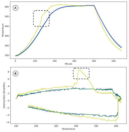
Figure 1. Example of cure cycle results. A: Temperature time series; B: rates diagram.

The objective of the proposed framework relies on assisting the officer during the validation, acting as an early-alerting system in the specific scenario. The framework works as follows. Firstly, it uses historical time series from cure cycles to train a regression model to predict future temperatures. Then, an online system monitors temperatures, forecasts them for the coming $$ 25 $$ min, and simultaneously compares predicted rates against requested ones. Whenever a discrepancy is identified, the operator is alerted. This way, it is possible to anticipate the anomaly for up to $$ 25 $$ min. Moreover, the system is adjusted through specific thresholds to classify the overall cure cycle very early. In fact, it compares all series forecasts with rate specifications and establishes when the overall process will fail. This additional functionality avoids a single sensor drift or failure invalidating the cure cycle. Still, it is mandatory to understand the work of other sensors. Practically, the system allows monitoring of the process in real-time to understand eventual failure or downtime of specific sensors and, in parallel, can decide, with anticipation, if the process will fail.

Let us demonstrate the functionality of online anomaly detection with an example. Figure 2 shows the procedure executed at the instant $$ i $$. The regression model predicts, taking advantage of the previous $$ 10 $$ temperatures, the following $$ 25 $$ for each series (see subfigure 2A). For each made prediction, starting from the temperature $$ t_i $$, the rate is calculated by comparing it with $$ t_{i-10} $$ following Equation (1) (with a backward step of 10 min, see subfigure 2B). When the computed rate does not meet the validation specifications (i.e., does not fall in the range between MIN LIMIT and MAX LIMIT of subfigure 2B), a single anomaly is detected at instant $$ i $$. The yellow series in subfigure 2B shows a set of anomalies due to rate values greater than the maximum allowed by the specifications. As one or more anomalies are identified, the framework compares the number of seen anomalies for all considered sensors to specific thresholds to establish the validity of the cure cycle. As soon as these anomalies are detected or exceed thresholds, the framework alerts the officer that can make decisions about the ongoing cycle without waiting for its end.

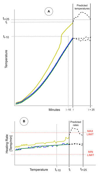
Figure 2. Example of anomaly detection at instant $$ i $$. A: predicted temperatures until instant $$ i+25 $$. B: corresponding rates compared with specifications.

Theoretical background

This subsection describes the background theories and concepts relevant to understanding the proposed methodology.

Long short term memory network

The LSTM ^[37] is a type of recurrent neural network (RNN). These networks can only keep a few previous stages in a sequence, making them ineffective for preserving longer data sequences. To undertake it, LSTM has additional features to memorize data sequences. A typical LSTM structure consists of a set of recurrently connected subnetworks, known as memory blocks. Each block is configured mainly by memory cell state, forget gate, input gate, and output gate. The central element, the memory cell, runs through the entire chain of blocks to add or remove information to the cell state with the support of gates. The forget gate decides what relevant information should be thrown away or kept. The input gate determines if it should update the information stored in the memory. Finally, the output gate learns when the stored information should be used. The structure of a memory block with one cell is shown in Figure 3.

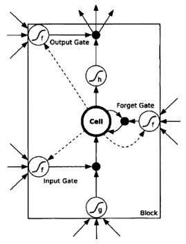
Figure 3. Structure of LSTM memory block with one cell ^[38].

The LSTM network works by identifying the correlation between the input and the output. Giving an input $$ x = (x_{1}, ... , x_{t}) $$, it calculates the network unit activation by iteratively processing the equations:

(2) $$ f_{t}=\sigma_{g} (W_{f}x_{t} + U_{f}h_{t-1} + b_{f}) $$

(3) $$ i_{t}=\sigma_{g} (W_{i}x_{t} + U_{i}h_{t-1} + b_{i}) $$

(4) $$ o_{t}=\sigma_{g} (W_{o}x_{t} + U_{o}h_{t-1} + b_{o}) $$

(5) $$ \tilde{c_{t}}=\sigma_{c} (W_{c}x_{t} + U_{c}h_{t-1} + b_{c}) $$

(6) $$ c_{t}=f_{t} \odot c_{t-1} + i_{t} \odot c_{t} $$

(7) $$ h_{t}=o_{t}\odot \sigma_{c}(C_{t}) $$

where the initial values are $$ c_{0} = 0 $$ and $$ h_{0} = 0 $$; $$ W $$, $$ U $$ and $$ b $$ denote, respectively, the weights of the input and recurrent connection and the bias vectors. Their subfix indicates the correspondence to the gate: $$ i $$ the input gate, $$ o $$ the output gate and $$ f $$ the forget gate and $$ c $$ the memory cell. These last three parameters are the ones that need to be learned during the training. $$ \sigma_{g} $$ represents the sigmoid activation function, $$ \sigma_{c} $$ the hyperbolic tangent activation function, $$ \odot $$ the Hadamard product (element-wise product) of the vectors, $$ f_{t}, i_{t}, o_{t} $$ and $$ \tilde{c_{t}} $$ the activation vectors of each gate, $$ c_{t} $$ the cell state vector and $$ h_{t} $$ the LSTM unit's hidden state vector, also known as the output vector.

LSTM has been chosen for the regression aim in this work due to its ability to process the overall data sequence, preserving important information.

Time series segmentation

Time series segmentation splits the series into homogeneous segments. It is used to add context information to time series. In particular, it establishes if temperatures undergo relevant changes (e.g., from the heating phase to stasis).

Among available segmentation models, three types can be identified: shape, statistic, and probabilistic methods. Statistical approaches use slope, mean, minimum or maximum metrics to identify segments. The probabilistic approach estimates segments based on the probability that a sample belongs to the same or a new segment. Finally, the shape approach uses the time series shape by resembling human viewing a plot ^[39]. This last model is implemented in this work; specifically, FLOSS is adopted ^[40].

FLOSS is a domain agnostic technique included in the STUMPY library, used for data mining in time series. It efficiently computes the matrix profile that keeps the z-normalized Euclidean distance between its nearest neighbor and any subsequence within the time series. FLOSS exploits this matrix and produces a companion time series called the Arc Curve (AC), which annotates the raw time series with information about the likelihood of a regime change at each location. The AC is essentially a pointer from an index to its nearest neighbor in the matrix index vector. The premise is that similar patterns should be included within the same regime and that the number of arc curves pointing between different regimes should be few. For example, using a time series with two regimes, the split would be where the minimum number of arc curves exists. However, this method has an edge situation in which no arc will live in the first sample in the time series. For this reason, the beginning of the time series must be compensated to not perform the segmentation at this point. So, the Corrected Arc Crossings (CAC) is defined as a metric of the number of overarching arc curves with the corrections for the edges, and as it is concerned with streaming data is strictly one-directional rather than bidirectional for the case of batch data. This metric is in the interval $$ [0, 1] $$, where a low value is few overarching curves, and high values are many. Figure 4 shows an example from a cure cycle sensor that measures temperatures. The image shows how the algorithm is able to identify a change in the series.

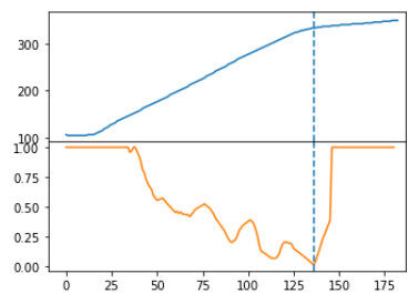
Figure 4. Example about temperature time series and corresponding CAC graph: a change is identified at minute $$ 136 $$.

Cure cycle validation methodology

The proposed solution mainly consists of two macro-phases. In the first one, a regression model (i.e., LSTM Neural Network) is trained through historical data from the cure cycle process in the aerospace industry. Then, the cure cycle validation phase exploits forecasting made by the LSTM generated in the previous step to validate the CC. This section details each phase.

LSTM neural network training

In this phase, a dataset of historical data of $$ 5 $$ types of composite material production is firstly pre-processed to adapt its format to the model input. In particular, the last $$ 10 $$ temperature values (i.e., $$ \{t_{i-1}, t_{i-2}, \dots, t_{i-10}\} $$) are inputted to the FLOSS algorithm, which returns a flag in $$ (0, 1) $$ as the semantic information about regime change associate to the series section. Finally, this information is attached to temperatures and inputted into the model. The output layer produces a vector of $$ 8 $$ values representing the predictions at the following instants: $$ \{t_i, t_{i+1}, t_{i+2}, t_{i+5}, $$$$ t_{i+10}, t_{i+15}, t_{i+20}, t_{i+25} \}$$.

The adopted LSTM has the following structure: one input layer, a hidden LSTM layer of $$ 64 $$ neurons with the default sigmoid activation function, followed by a dropout of $$ 0.3 $$ and, finally, an output layer that makes the prediction. The model training was compiled with a mean squared error (MSE) loss function to calculate the difference between real and predicted values and with Adam optimizer using the default learning rate. Details about achieved performance are reported in the Results Section.

Cure cycle validation

At each timestamp (i.e., minute), temperatures forecasted by the model trained in the previous phase are adopted to establish whether the anomaly will occur. More in detail, at each timestamp $$ i $$, the framework passes to the LSTM model the last 10 temperatures and the FLOSS information at that instant. As a result, the model produces the prediction of $$ 8 $$ values that reaches $$ 25 $$ min after $$ i $$ (i.e., the forecasts). For each forecast, a rate is calculated with a backward step of $$ 10 $$ min¹ by utilizing the temperature value at the $$ 10th $$ precedent minute and the predicted value. The rate values are then validated through the Cure Verification Algorithm.

¹This value derives from validation criteria.

Essentially, the cure cycle validation phase can be summarized as follows (see Figure 5):

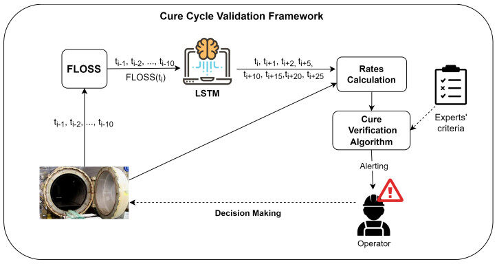
Figure 5. Cure Cycle Validation workflow.

● Last $$ 10 $$ temperatures are input for the FLOSS algorithm;

● The FLOSS output, together with the last $$ 10 $$ temperatures, is submitted to the LSTM model;

● The LSTM model forecasts up to $$ 25 $$ min ahead;

● Forecasts are input for heating rate calculation. Such values measure the increase or decrease rates of curves and are explicitly adopted by experts to make cure cycle validations;

● The Cure Verification Algorithm compares future rates with experts' criteria, decides if an operator needs alerting by comparing the number of anomalies with fixed thresholds, and classifies the cycle as valid or invalid.

Cure Verification Algorithm

The proposed Cure Verification Algorithm, mainly responsible for the cure cycle validation, is shown in Figure 6.

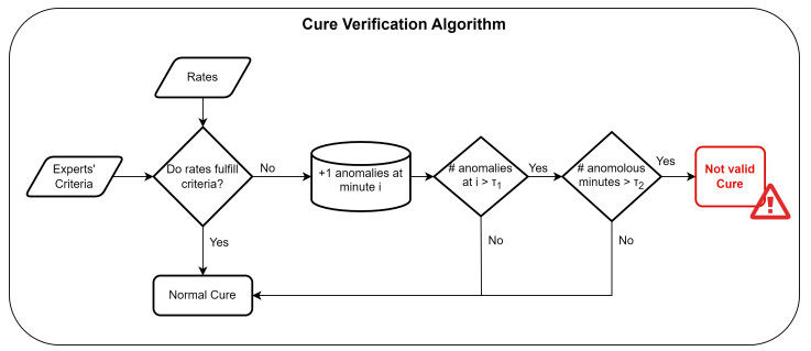
Figure 6. Cure Verification Algorithm.

Let us start again distinguishing between anomaly and invalid cure cycle. The first is identified when a difference between predicted rates and experts' criteria arises. Conversely, a cycle is considered invalid when the number of anomalies exceeds specific thresholds. In this sense, two defined thresholds measure, respectively, the number of recognized anomalies at each instant $$ i $$ (i.e., $$ \tau_1 $$) and the number of instants for which there are more than $$ \tau_1 $$ anomalies (i.e., $$ \tau_2 $$). So, the algorithm makes the following checks:

● At each instant $$ i $$, the rate evaluated through real and predicted temperatures is compared with the defined experts' criteria. If criteria are not passed, the number of anomalies for the minute $$ i $$ is incremented.

● At each instant $$ i $$, the number of minutes $$ N $$ having more than $$ \tau_1 $$ forecasted anomalies is compared with $$ \tau_2 $$. If $$ N > \tau_2 $$, the operator is alerted about the invalid cure cycle.

RESULTS

This section details the experimentation carried out to evaluate the proposed framework in terms of invalid cure cycle identification, on real data. The following sections describe the adopted dataset, evaluation measures, and validation processes.

Discussion

The spread of Industry 4.0 allowed manufacturers the adoption of new technologies (e.g., smart sensors). Such equipment produces a consistent amount of real-time data that gives many data analysis opportunities that could feed learning models or decision support systems.

This work, developed during activities of the project Leonardo 4.0, proposes an early cure cycle validation based on a deep learning model through real data. First, an LSTM is trained with historical data regarding a cure cycle for composite material production from autoclaves. The resulting model predicts future temperatures at each step (i.e., minute) and compares them with validation criteria. Through that criteria, the system continuously monitors process data and early informs the quality control officer about drifting series (regarding specific sensors) or, more in general, of inadequateness of the ongoing cure cycle. The officer can decide to make suitable decisions that can positively impact not only the production time and the final product, but also the environment.

Experiments made on a real dataset provided by Leonardo s.p.a. reveal a good capacity of the framework to discern between valid and invalid cures with consistent anticipation.

Although the proposal experimented with a single case study, the LSTM originally used the output of the FLOSS algorithm as the contextual information of the time series. This choice and the exhibited performance support the hypothesis that the method can be used in other contexts tuning thresholds and providing other time series.

Declarations

REFERENCES

1. Abubakr M, Abbas AT, Tomaz I, et al. Sustainable and smart manufacturing: an integrated approach. Sustainability 2020;12:2280.
2. M Mabkhot M, Ferreira P, Maffei A, et al. Mapping industry 4.0 enabling technologies into united nations sustainability development goals. Sustainability 2021;13:2560.
3. Hundman K, Constantinou V, Laporte C, Colwell I, Soderstrom T. Detecting spacecraft anomalies using lstms and nonparametric dynamic thresholding. In: Proceedings of the 24th ACM SIGKDD International Conference on Knowledge Discovery & Data Mining; 2018. pp. 387-95.
4. Rincon-Yanez D, Crispoldi F, Onorati D, et al. Enabling a semantic sensor knowledge approach for quality control support in cleanrooms. In: International Semantic Web Conference. vol. 2980; 2021.
5. Cao Q, Giustozzi F, Zanni-Merk C, de Bertrand de Beuvron F, Reich C. Smart condition monitoring for industry 4.0 manufacturing processes: An ontology-based approach. Cybernetics and Systems 2019;50:82-96.
6. Zhou B, Svetashova Y, Gusmao A, et al. SemML: Facilitating development of ML models for condition monitoring with semantics. J Web Semant 2021;71:100664.
7. Weese M, Martinez W, Megahed FM, Jones-Farmer LA. Statistical learning methods applied to process monitoring: An overview and perspective. J Qual Technol 2016;48:4-24.
8. Zhang C, Song D, Chen Y, et al. A deep neural network for unsupervised anomaly detection and diagnosis in multivariate time series data. In: Proceedings of the AAAI Conference on Artificial Intelligence. vol. 33; 2019. pp. 1409-16.
9. Fenza G, Gallo M, Loia V. Drift-aware methodology for anomaly detection in smart grid. IEEE Access 2019;7:9645-57.
10. Pittino F, Puggl M, Moldaschl T, Hirschl C. Automatic anomaly detection on in-production manufacturing machines using statistical learning methods. Sensors 2020;20:2344.
11. Wu D, Jiang Z, Xie X, et al. LSTM learning with Bayesian and Gaussian processing for anomaly detection in industrial IoT. IEEE Trans Ind Inf 2019;16:5244-53.
12. Ergen T, Kozat SS. Unsupervised anomaly detection with LSTM neural networks. IEEE Trans Neural Netw Learn Syst 2019;31:3127-41.
13. Siami-Namini S, Tavakoli N, Namin AS. A comparison of ARIMA and LSTM in forecasting time series. In: 2018 17th IEEE International Conference on Machine Learning and Applications (ICMLA). IEEE; 2018. pp. 1394-401.
14. Park BE, Kim JS, Lee JK, Lee IB. Anomaly detection in a hyper-compressor in low-density polyethylene manufacturing processes using WPCA-based principal component control limit. Korean J Chem Eng 2020;37:11-18.
15. Arena E, Corsini A, Ferulano R, et al. Anomaly detection in photovoltaic production factories via monte carlo pre-processed principal component analysis. Energies 2021;14:3951.
16. Falanga M, De Lauro E, Petrosino S, Rincon-Yanez D, Senatore S. Semantically enhanced IoT-oriented seismic event detection: an application to Colima and Vesuvius volcanoes. IEEE Internet Things J 2022; doi: 10.1109/JIOT.2022.3148786.
17. Mokhtari S, Abbaspour A, Yen KK, Sargolzaei A. A machine learning approach for anomaly detection in industrial control systems based on measurement data. Electronics 2021;10:407.
18. Ahamed J, Koli AM, Ahmad K, Jamal MA, Gupta BB. CDPS-IoT: cardiovascular disease prediction system based on iot using machine learning. IJIMAI 2022;7:78-86.
19. Basora L, Olive X, Dubot T. Recent advances in anomaly detection methods applied to aviation. Aerospace 2019;6:117.
20. Nanduri A, Sherry L. Anomaly detection in aircraft data using Recurrent Neural Networks (RNN). In: 2016 Integrated Communications Navigation and Surveillance (ICNS). IEEE; 2016. pp. 5C2-.
21. Mori R. Anomaly detection and cause analysis during landing approach using recurrent neural network. J Aero Inf Syst 2021;18:679-85.
22. Ding N, Ma H, Gao H, Ma Y, Tan G. Real-time anomaly detection based on long short-Term memory and Gaussian Mixture Model. Computers & Electrical Engineering 2019;79:106458.
23. Lejon E, Kyösti P, Lindström J. Machine learning for detection of anomalies in press-hardening: Selection of efficient methods. Procedia Cirp 2018;72:1079-83.
24. Petković D. Prediction of laser welding quality by computational intelligence approaches. Optik 2017;140:597-600.
25. Quatrini E, Costantino F, Di Gravio G, Patriarca R. Machine learning for anomaly detection and process phase classification to improve safety and maintenance activities. J Manuf Syst 2020;56:117-32.
26. Carlone P, Aleksendrić D, Rubino F, Ćirović V. Artificial neural networks in advanced thermoset matrix composite manufacturing. In: Ni J, Majstorovic VD, Djurdjanovic D, editors. Proceedings of 3rd International Conference on the Industry 4.0 Model for Advanced Manufacturing. Cham: Springer International Publishing; 2018. pp. 78-88.
27. Zhang C, Ji W. Edge computing enabled production anomalies detection and energy-efficient production decision approach for discrete manufacturing workshops. IEEE Access 2020;8:158197-207.
28. Okeke D, Musa SM. Energy management and anomaly detection in condition monitoring for industrial internet of things using machine learning. In: 2021 International Conference on Informatics, Multimedia, Cyber and Information System (ICIMCIS. IEEE; 2021. pp. 65-68.
29. Shahbazi S, Salloum M, Kurdve M, Wiktorsson M. Material efficiency measurement: empirical investigation of manufacturing industry. Procedia Manufacturing 2017;8:112-20.
30. Park M, Jeong J. Design and Implementation of Machine Vision-Based Quality Inspection System in Mask Manufacturing Process. Sustainability 2022;14:6009.
31. Crawford B, Sourki R, Khayyam H, S Milani A. A machine learning framework with dataset-knowledgeability pre-assessment and a local decision-boundary crispness score: An industry 4.0-based case study on composite autoclave manufacturing. Computers in Industry 2021;132:103510.
32. Chen YX, Wang LC, Chu PC. A recipe parameter recommendation system for an autoclave process and an empirical study. Procedia Manufacturing 2020;51:1046-53.
33. Golkarnarenji G, Naebe M, Badii K, et al. Support vector regression modelling and optimization of energy consumption in carbon fiber production line. Computers & Chemical Engineering 2018;109:276-88.
34. Lindemann B, Jazdi N, Weyrich M. Anomaly detection and prediction in discrete manufacturing based on cooperative LSTM networks. In: 2020 IEEE 16th International Conference on Automation Science and Engineering (CASE); 2020. pp. 1003-10.
35. Lindemann B, Fesenmayr F, Jazdi N, Weyrich M. Anomaly detection in discrete manufacturing using self-learning approaches. Procedia CIRP 2019;79:313-18.
36. Bai Y, Xie J, Wang D, Zhang W, Li C. A manufacturing quality prediction model based on AdaBoost-LSTM with rough knowledge. Computers & Industrial Engineering 2021;155:107-227.
37. Hua Y, Zhao Z, Li R, et al. Deep learning with long short-term memory for time series prediction. IEEE Commun Mag 2019;57:114-19.
38. Luo X, Li D, Yang Y, Zhang S. Spatiotemporal traffic flow prediction with KNN and LSTM. J Adv Trans 2019;2019.
39. Svensson M. Unsupervised Segmentation of Time Series Data; 2021.
40. Gharghabi S, Ding Y, Yeh CCM, et al. Matrix profile Ⅷ: domain agnostic online semantic segmentation at superhuman performance levels. In: 2017 IEEE international conference on data mining (ICDM). IEEE; 2017. pp. 117-26.
Cite This Article
Export citation file: BibTeX | RIS
OAE Style
Bangerter ML, Fenza G, Gallo M, Volpe A, Caminale G, Gallo N, Leone F. A case study in smart manufacturing: predictive analysis of cure cycle results for a composite component. J Smart Environ Green Comput 2022;2:76-89. http://dx.doi.org/10.20517/jsegc.2022.11
AMA Style
Bangerter ML, Fenza G, Gallo M, Volpe A, Caminale G, Gallo N, Leone F. A case study in smart manufacturing: predictive analysis of cure cycle results for a composite component. Journal of Smart Environments and Green Computing. 2022; 2(3): 76-89. http://dx.doi.org/10.20517/jsegc.2022.11
Chicago/Turabian Style
Bangerter, Micaela Lucia, Giuseppe Fenza, Mariacristina Gallo, Alberto Volpe, Gianfranco Caminale, Nicola Gallo, Fabrizio Leone. 2022. "A case study in smart manufacturing: predictive analysis of cure cycle results for a composite component" Journal of Smart Environments and Green Computing. 2, no.3: 76-89. http://dx.doi.org/10.20517/jsegc.2022.11
ACS Style
Bangerter, ML.; Fenza G.; Gallo M.; Volpe A.; Caminale G.; Gallo N.; Leone F. A case study in smart manufacturing: predictive analysis of cure cycle results for a composite component. . J. Smart. Environ. Green. Comput. 2022, 2, 76-89. http://dx.doi.org/10.20517/jsegc.2022.11
About This Article
Special Issue
Copyright
Data & Comments
Data
Cite This Article 9 clicks
Like This Article 25
likes
Comments
Comments must be written in English. Spam, offensive content, impersonation, and private information will not be permitted. If any comment is reported and identified as inappropriate content by OAE staff, the comment will be removed without notice. If you have any queries or need any help, please contact us at support@oaepublish.com.